Support vector machine is a type of supervised machine learning that is used for both classification and regression, but classification is preferable.
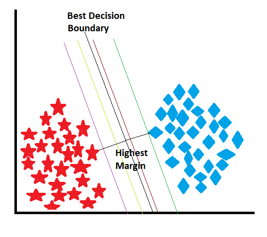
We know about linear regression and logistic regression. In linear regression, the model draws a multiple-fitted line and chooses one line as the best-fit line, which covers the maximum number of data points. In a logistic regression model, it draws an S-shaped curve that lies between 0 and 1. However, Support Vector Machines (SVM) are also similar to linear regression and logistic regression. SVM also draws multiple lines at the back end and chooses one as the best decision boundary. It also draws a curve. But the main difference is the shape of the line.
SVM draws a straight line as a decision boundary when the data is linearly separable, which means there is a clear gap or space between the two classes that can be separated by a straight line. A linear decision boundary is the most straightforward option when the data can be separated. On the other hand, SVM uses a non-linear curve as a decision boundary when the data is not linearly separable, which means there is no straight line that can perfectly separate the two classes.
How does SVM work?
When the model receives the data, it draws multiple-decision boundaries, also known as a hyperplane, and chooses the best one. After assigning the decision boundary, the model starts to find the nearest data points for each class and draws the imaginary hyperplane from those points, which is called the support vector. The distance between the support vector and the decision boundary is known as the margin, and the model always tries to maximize the margin. Let’s explore these concepts with appropriate images and descriptions.
Actual Decision Boundary (Hyperplane):
The actual decision boundary, also known as the hyperplane, is the “real” line (in 2D) or “real” flat surface (in higher dimensions) that separates the data points belonging to different classes. In a binary classification problem, the hyperplane is the line or surface that separates the positive class from the negative class with the maximum margin.
—————————————————————————————————————————————————————————————————-
Imaginary Hyperplanes Travelling from Support Vectors:
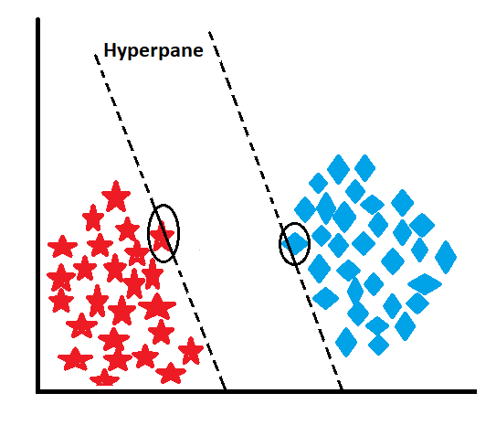
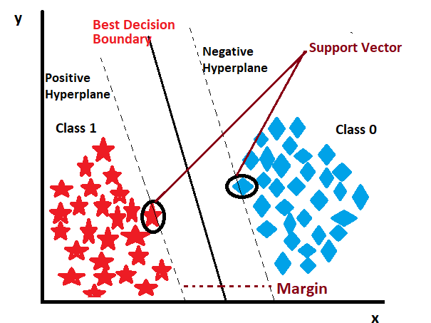
In SVM, the support vectors are the data points that are closest to the actual decision boundary. They play a crucial role in defining the hyperplane. For each support vector, there is an “imaginary” hyperplane associated with it. These imaginary hyperplanes “travel” from the support vectors toward the actual decision boundary.
In a 2-dimensional space, these imaginary hyperplanes are lines that originate from the support vectors and point toward the actual decision boundary. These lines help define the margin, which is the distance between the imaginary hyperplanes in both classes. The actual decision boundary is chosen in such a way that it maximizes the margin, which is equivalent to finding the hyperplane that separates the imaginary hyperplanes from the positive and negative classes with the maximum margin. These imaginary hyperplanes represent the influence of the support vectors on the decision boundary. The distance between the imaginary hyperplanes and the actual decision boundary is essential for determining the optimal hyperplane, and it directly affects the margin and classification performance of the SVM classifier.
—————————————————————————————————————————————————————————————————-
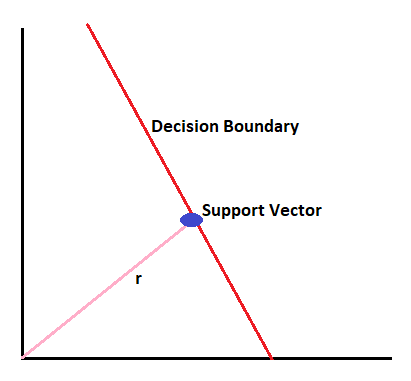
Support Vector:
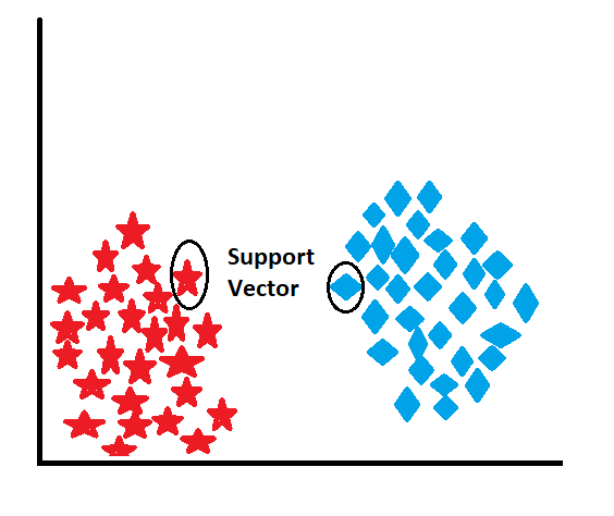
Support vectors are the data points from the training set that are closest to the decision boundary (hyperplane) in SVM classification. These are the critical data points that define the margin of separation between the classes. Support vectors are essential because they play a significant role in determining the optimal hyperplane. They influence the positioning and orientation of the decision boundary, as SVM aims to maximize the margin between the support vectors of different classes.
—————————————————————————————————————————————————————————————————-
Margin:
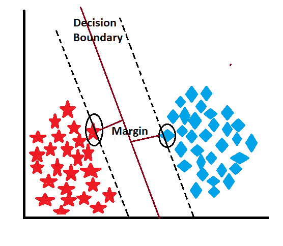
In the context of Support Vector machines (SVM), the margin refers to the separation between the decision boundary (hyperplane) and the closest data points from each class. The goal of SVM is to maximize this margin, as a wider margin indicates better generalization and robustness of the classifier. Maximizing the margin helps reduce the risk of misclassification and improves the ability of the model to correctly classify new, unseen data points.
Types of Margin:
Hard Margin:
- In Hard Margin SVM, the goal is to find a decision boundary that perfectly separates the two classes without any misclassifications.
- This means that the margin is maximized while ensuring that all the data points are correctly classified.
- Hard Margin SVM works only when the data is linearly separable, i.e., a straight line can completely separate the two classes.
Soft Margin:
- In Soft Margin SVM, we allow some misclassifications to find a decision boundary when the data is not perfectly separable.
- It introduces a “slack variable” (ξ) for each data point, which measures the degree of misclassification, or how far the data point is on the wrong side of the margin.
- The objective is to minimize the misclassifications (slack variables) while still maximizing the margin as much as possible.
- Soft Margin SVM is more flexible and can handle non-linearly separable data by allowing some errors.
If the data is linearly separable (no overlapping between classes) and you want a strict, clean separation without any errors, you can use Hard Margin SVM.
If the data is not perfectly separable (some overlap between classes) or you want a more robust model that can tolerate some errors and outliers, you should consider Soft Margin SVM.
C Parameter:
In Soft Margin SVM, there is a regularization parameter called “C” that controls the trade-off between maximizing the margin and allowing misclassifications. A smaller C value emphasizes a wider margin, allowing more misclassifications, while a larger C value prioritizes a smaller margin, which reduces misclassifications.
—————————————————————————————————————————————————————————————————-
Hyperplane:
Positive Hyperplane:
A positive hyperplane is the decision boundary that separates one class (e.g., class A) from the other class (e.g., class B) in SVM classification. It is called “positive” because it is on the side of the class whether we are interested in classifying correctly.
Negative Hyperplane:
In SVM classification, the negative hyperplane is the decision boundary that separates the other class (e.g., class B) from the class of interest (e.g., class A). It is called “negative” because it is on the side of the class that we want to classify as the “other” class.
—————————————————————————————————————————————————————————————————-
Now let’s see how it predicts.
To find the class for any input, we need to find the dot product of that point. The dot product can be defined as the projection of one vector onto another.
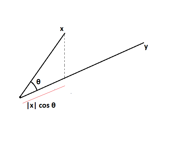
xy= |x|* cos θ * |y|
While finding the dot product, we only consider the projection and don’t require magnitude. Since we take the unit vector of another vector.
xy = |x|* cos θ * unit vector of y
Suppose a model learns the pattern of data and draws a decision boundary. Now it’s time to predict. Suppose we have ‘p’ input and need to find which class it belongs to. To find this, first of all, we need to draw one more vector named ‘q’, which lies at such a position that is perpendicular to the decision boundary and originates. Let’s apply the dot product to p and q.
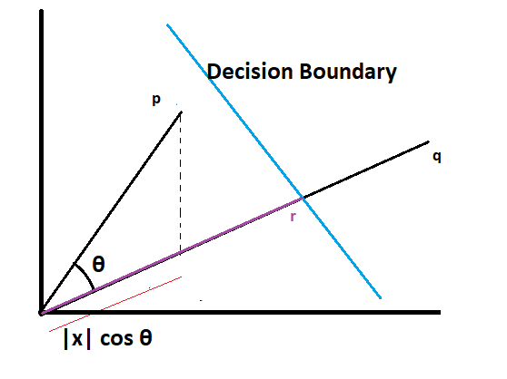
The dot product of pq = |p|* cos θ * the unit vector of q
Now combine this dot product value with bias and compare it with the r-value, which is nothing but the threshold value, to decide the class of input.
pq + bias = r
If the answer is less than r, then we can say the input ‘p’ point lies on the left-hand side of the class.
If the answer is greater than r, then we can say input ‘p’ lies on the right-hand side of the class.
If the answer comes equal to r, then we can say that the point lies on the decision boundary, and by default, it assumes the right-hand side class.
How do I select the r?
Determining the value of the threshold ‘r’ in Support Vector Machines (SVM) is an important task and can be influenced by various factors. The specific method to determine ‘r’ depends on the problem and the requirements of the classification task. Here are some common approaches to determining the value of ‘r’:
Manual Tuning:
- In some cases, the threshold ‘r’ can be set manually based on prior knowledge or domain expertise.
- Data scientists or machine learning practitioners may try different values of ‘r’ and evaluate the performance of the SVM classifier on a validation set to find the best value.
Grid Search:
- For a more systematic approach, a grid search can be employed to explore a range of ‘r’ values.
- The data scientist defines a range of possible values for ‘r’, and the SVM classifier is trained and evaluated using each value in the grid.
- The r-value that results in the best performance (e.g., highest accuracy or F1-score) on the validation set is chosen as the final threshold.
Cross-Validation:
- Cross-validation is a widely used technique to assess the performance of a model on different subsets of data.
- By performing cross-validation with different ‘r’ values, the data scientist can get an idea of how the SVM performs with various thresholds.
- The r-value that provides the best average performance across the cross-validation folds is selected.
Automatic Tuning Algorithms:
Some libraries or frameworks provide automatic tuning algorithms (e.g., GridSearchCV in Scikit-Learn) that can search for the best r-value using techniques like grid search or random search. These algorithms automate the process of finding the optimal ‘r’ value and save time and effort.
In this way, we can find the class for any input.
—————————————————————————————————————————————————————————————————-
There are two types of SVM.
- Linear SVM
- non-linear SVM.
Linear SVM:
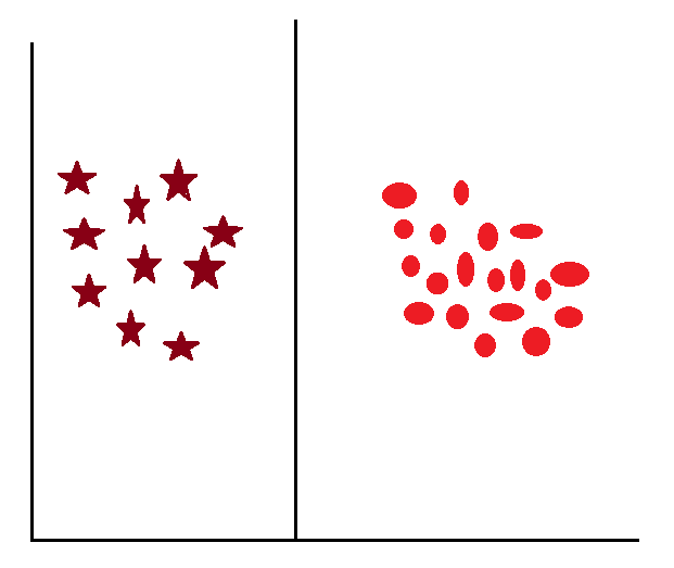
Here, the model receives data that is linearly separate; the difference between classes is very easily apparent. That means here, the model doesn’t need to make much effort to separate the data to draw a decision boundary. Let’s see some examples of linearly separable data.
If there are two linearly separable classes.
—————————————————————————————————————————————————————————————————-
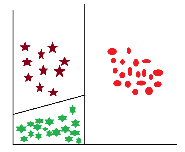
If there are three linearly separable classes
—————————————————————————————————————————————————————————————————-
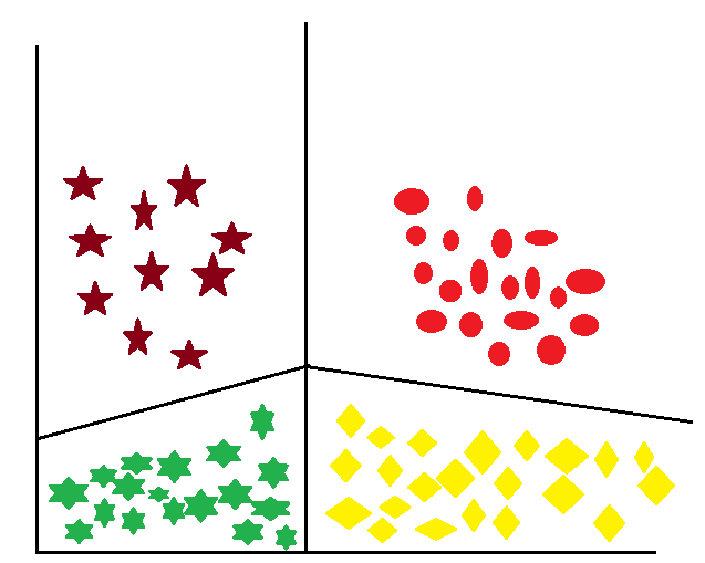
If there are four linearly separable classes
—————————————————————————————————————————————————————————————————-
Non-linear SVM:
However, most of the time, models receive data where classes are not easily separated; instead, we can say that the data points of different classes are mixed, making it hard to separate them and draw the decision boundary among these classes. Let’s take some examples:
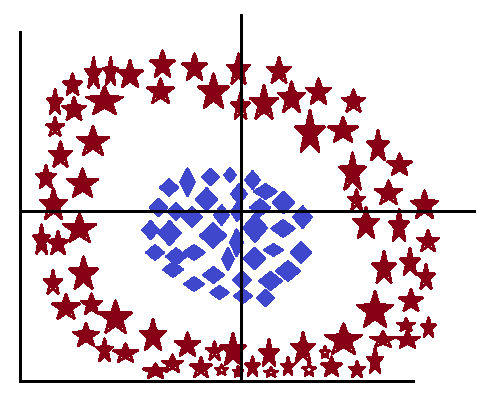
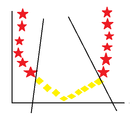
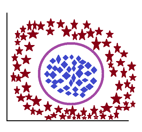
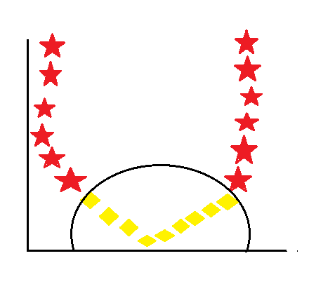
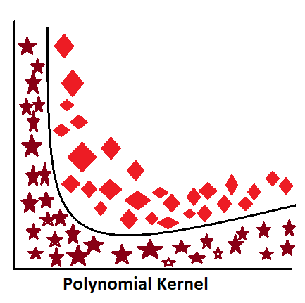
To overcome this, we use Kernel. A kernel is a mathematical trick used to draw a decision boundary in complex and nonlinearly separable data. In this Kernel increase the increased dimensional space, since it’s now possible to find a hyperplane, also known as a decision boundary, that can separate the groups of classes easily and efficiently. However, the hyperplane created, will not be a straight line; instead, it will be a curved line.
let’s see how the curve line divides the similar class.
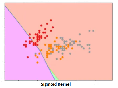
There are different types of kernels, which are listed below.
Polynomial Kernel:
—————————————————————————————————————————————————————————————————-
Sigmoid Kernel:
—————————————————————————————————————————————————————————————————-
RBF Kernel:

—————————————————————————————————————————————————————————————————-