It is a supervised machine learning algorithm that is used to find the linear relation between one dependent and one or more independent variables. That means it is used to find the dependency between input variables and output variables. If there is only one independent variable, then it is known as simple linear regression, and if there are more than one independent variables, then it is known as multiple linear regression.
Simple linear regression: y=m*x+c.
| x | y |
| 1 | 10 |
| 2 | 20 |
| 3 | 30 |
Simple Linear Regression.
multiple linear regression: y= m1*x1+m2*x2………..mi*xi +b.
| x1 | x2 | x3 | x4 | x5 | y |
| 1 | 4 | 7 | 10 | 13 | 100 |
| 2 | 5 | 8 | 11 | 14 | 200 |
| 3 | 6 | 9 | 12 | 15 | 300 |
Multiple Linear Regression.
Where,
y= Dependent variable/ output variable/ targets/ supervisions.
x=Independent variable/ input variable/ predictors .
m= slope.
c= intercept.
In following figure we can see what is slope and what intercept is.
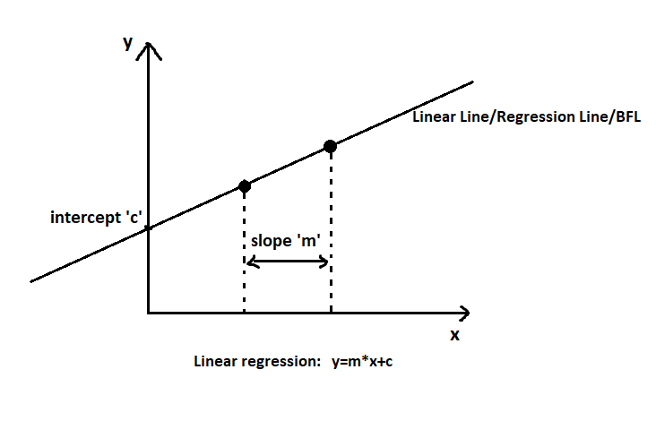
Slope is nothing but the difference between two adjacent variables on the linear line, and Intercept is the area from where the linear line travels. (Intercept the axis.)
Linear regression’s dependent variable must be in continuous order because whatever prediction is going on is in the form of a continuous value. For example, price prediction, age prediction, amount prediction, and independent variables can be in any form, like continuous or categorical. In real time, while using machine learning and solving continuous value-related problems, we prefer linear regression because it is a statistical algorithm that helps to explain the behavior of each parameter with respect to the dependent variable. And if there is any requirement at the end, like we need to explain all the details about each features, like how each parameter is related to the target variable as well as with others, whether it is it going to contribute to model performance or not, etc. then we should go with linear regression.
Linear regression draws multiple linear lines in the spread of data and chooses one line as the best linear line also known as Best Fit Line (BFL), which travels from such an area where the maximum number of data points will be covered. If maximum data points get covered by that best fit line, then we can say that dataset is linear, or tends towards linearity. But if a linear line doesn’t cover the maximum number of data points, we can conclude that the spread of data is not in linear form. We are going to see this topic in depth in terms of linearity, first assumption of linear regression.
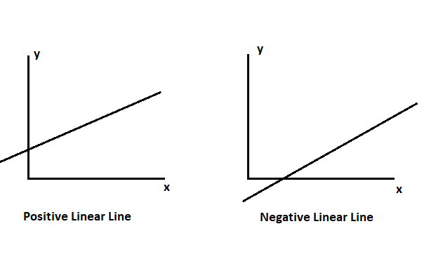
The best fit line is also known as a linear line, regression line, or prediction line. There are two types of BFL: positive BFL and negative BFL.
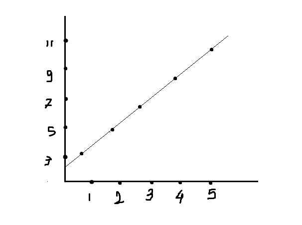
Now let’s see how we can predict by using the linear regression formula: Y=m*x+c.
| x | y |
| 1 | 3 |
| 2 | 5 |
| 3 | 7 |
| 4 | 9 |
| 5 | 11 |
| 7 | ? |
y=m*x+c and we want prediction for 7.
Slope (m):
(x1, y1) = (1, 3)
(x2, y2) = (2, 5)
(x3, y3) = (3, 7)
(x4, y4) = (4, 9)
(x5, y5) = (5, 11)
Calculate the means:
x̄ = (1 + 2 + 3 + 4 + 5) / 5 = 3
ȳ = (3 + 5 + 7 + 9 + 11) / 5 = 7
Calculate the differences:
Δx1 = x1 – x̄ = 1 – 3 = -2
Δx2 = x2 – x̄ = 2 – 3 = -1
Δx3 = x3 – x̄ = 3 – 3 = 0
Δx4 = x4 – x̄ = 4 – 3 = 1
Δx5 = x5 – x̄ = 5 – 3 = 2
Δy1 = y1 – ȳ = 3 – 7 = -4
Δy2 = y2 – ȳ = 5 – 7 = -2
Δy3 = y3 – ȳ = 7 – 7 = 0
Δy4 = y4 – ȳ = 9 – 7 = 2
Δy5 = y5 – ȳ = 11 – 7 = 4
Calculate the numerator:
Σ(Δx * Δy) = (Δx1 * Δy1) + (Δx2 * Δy2) + (Δx3 * Δy3) + (Δx4 * Δy4) + (Δx5 * Δy5)
= (-2 * -4) + (-1 * -2) + (0 * 0) + (1 * 2) + (2 * 4)
= 8 + 2 + 0 + 2 + 8
= 20
Calculate the denominator:
Σ(Δx^2) = (Δx1^2) + (Δx2^2) + (Δx3^2) + (Δx4^2) + (Δx5^2)
= (-2^2) + (-1^2) + (0^2) + (1^2) + (2^2)
= 4 + 1 + 0 + 1 + 4
= 10
Calculate the slope ‘m’:
m = Σ(Δx * Δy) / Σ(Δx^2)
= 20 / 10
= 2
Intercept:
c = ȳ – m * x̄
x̄ = 3
ȳ = 7
Using the slope value we obtained earlier, m = 2, we can calculate the intercept ‘c’:
c = ȳ – m * x̄
= 7 – 2 * 3
= 7 – 6
= 1
Plugging these values into the equation, we get:
x=7
m=2
c=15
y = 2 * x + 1
= 2 * 7 + 1
= 14 + 1
y= 15
In this way, linear regression runs and predicts for unseen input.
Linear Regression is a parametric algorithm, which means it should obey some assumptions to improve training and increase the performance of the model. These are listed below.
- Linearity.
- Independence.
- No – Multicollinearity.
- Normality.
- Homoscedasticity.
Linearity:
Data should be linear, which means whatever independent variables are in the dataset should be linearly relates with the dependent variable. The spread of data should be in linear format, whatever it would be positively linear or negatively linear.
The linear spread could be in 1st and 3rd quadrants, or 2nd and 4th quadrants. How? Let’s see.
We have four quadrants in which we can see the spread of the data set.
1st Quadrants = +ve spread2nd Quadrants = -ve spread
3rd Quadrants = +ve spread
4th Quadrants = -ve spread
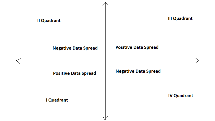
So if we get data spread in 1st & 3rd quadrants then whatever data we get that data we can say, it is in positive linear spread. Data lies in 2nd & 4th also give linear form of data but it is in negative spread. Beyond this group if we get data in any quadrants, then that data we can say, not in linear format. And last one, if we get data in all quadrants then we can say, it is cloudy data.
Mathematically, if we want to see the linearity, we can find it by using the Rxy value, which is also known as the coefficient of correlation. The R value gives information about the predictors.
- If Rxy = 1 or -1 then we can say that predictor is best one for model.
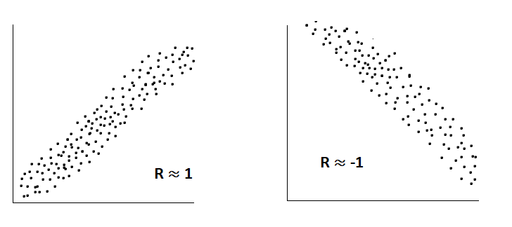
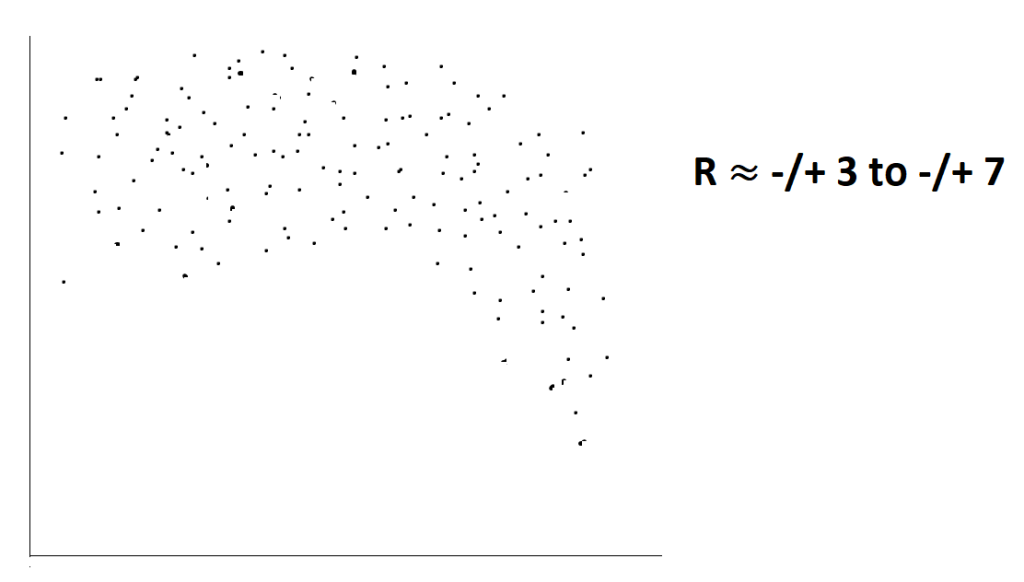
- If Rxy = -3 to 7 or 3 to 7 average predictors.
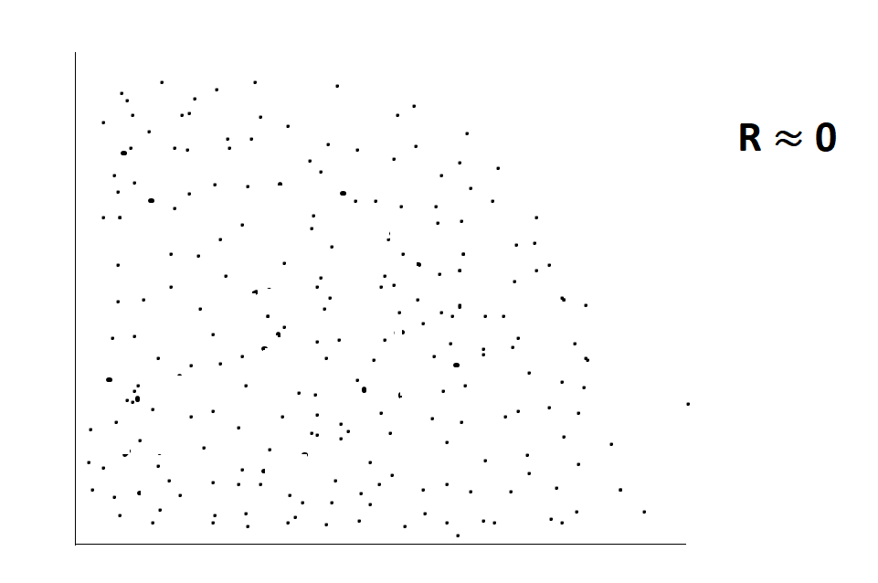
- If Rxy = 0 Bad predictors.
Formula for Rxy = Σ((xi – x̄)(yi – ȳ)) / sqrt(Σ(xi – x̄)² * Σ(yi – ȳ)²)
- xi = independent variable.
- x̄ = mean of independent variable.
- yi = dependent variable.
- ȳ = mean of dependent variable.
It is also known as: Covariance / standard deviation.
Covariance: Spread of data from it mean.
Σ((xi – x̄)(yi – ȳ))/ n-1.
Standard deviation: deviation of covariance
sqrt(Σ(xi – x̄)² * Σ(yi – ȳ)²)/n-1.
Let’s see how Rxy value calculate:
Calculate the means of x and y:
x̄ = (1 + 2 + 3 + 4 + 5) / 5 = 3
ȳ = (3 + 5 + 7 + 9 + 11) / 5 = 7
Calculate the differences between each x value and the mean of x (Δx) and each y value and the mean of y (Δy) for each data point:
For x:
Δx1 = x1 – x̄ = 1 – 3 = -2
Δx2 = x2 – x̄ = 2 – 3 = -1
Δx3 = x3 – x̄ = 3 – 3 = 0
Δx4 = x4 – x̄ = 4 – 3 = 1
Δx5 = x5 – x̄ = 5 – 3 = 2
For y:
Δy1 = y1 – ȳ = 3 – 7 = -4
Δy2 = y2 – ȳ = 5 – 7 = -2
Δy3 = y3 – ȳ = 7 – 7 = 0
Δy4 = y4 – ȳ = 9 – 7 = 2
Δy5 = y5 – ȳ = 11 – 7 = 4
Calculate the numerator Σ(Δx * Δy):
Σ(Δx * Δy) = (-2 * -4) + (-1 * -2) + (0 * 0) + (1 * 2) + (2 * 4) = 8 + 2 + 0 + 2 + 8 = 20
Calculate the sum of the squared differences for x (Σ(Δx^2)):
Σ(Δx^2) = (-2^2) + (-1^2) + (0^2) + (1^2) + (2^2) = 4 + 1 + 0 + 1 + 4 = 10
Calculate the sum of the squared differences for y (Σ(Δy^2)):
Σ(Δy^2) = (-4^2) + (-2^2) + (0^2) + (2^2) + (4^2) = 16 + 4 + 0 + 4 + 16 = 40
Calculate the square root of Σ(Δx^2) and Σ(Δy^2):
sqrt(Σ(Δx^2)) = sqrt(10) ≈ 3.16
sqrt(Σ(Δy^2)) = sqrt(40) ≈ 6.32
Calculate Rxy using the formula:
Rxy = Σ(Δx * Δy) / (sqrt(Σ(Δx^2)) * sqrt(Σ(Δy^2)))
= 20 / (3.16 * 6.32)
≈ 20 / 19.965
≈ 1.001
The correlation coefficient (Rxy) is approximately equal to 1.001, indicating a strong positive correlation between the variables x and y in this dataset.
Independency:
This assumption states that there should be a dependency between only independent variables and dependent variables, not between independent variables. If in the model we see dependency between independent variables, then we are just increasing our computational power, not the performance of model. Suppose we have 1000 recorded data set, and 7 independent variables in that, now suppose in that one variable is totally depend on one another variable. Now we know that dependency between independent variable is not useful, still if we try to run the model then model run on that particular variable for total 1000 times, because our dataset size is 1000. By this, we can assume that, we just increasing the complexity, increasing the time, use extra memory, increasing the cost of model only because of use of such dependency in independent variable.
For example in bank loan dataset, there is one column named with family income, which combines all family members income, suppose there is one more column which is separately defined for husband income or wife income, now let’s understand what actually problem we get here. As we get the loan dataset, there is one big column which combine all family members’ income, so there is no need to declare each and every members income individually. Because at the end it goes to sum all, so therefore if we found such extra column then it just useless feature and this feature not going to give any contribution to model performance.
To find a dependency between independent variables, we can use Rxy value. In this, we can see the comparison of each independent variable based on dependency in between them.
Rxy value comparison between independent variable:-
- 0: no relationship between two variable.
- 1: strong relationship..
- -7 to 7: relationship present.
- -3 to 3: poor relationship.
If we found dependency between independent variable, we can do two things: Check both independent variable’s R value with respect to dependent variable and choose one of them which gives the highest R value and delete another one. Or join these two and make a new one.
No – Multicollinearity.
No multicollinearity means there should be a high correlation between independent and dependent variables only. Whatever the requirement of multicollinearity should be in between dependent and independent only.
To find out if there is any multicollinearity between independent variables, there are two techniques.
- VIF.
- Tolerance.
- VIF (Variance Inflation Factor) :
Formula: 1/1 – r^2. ( r^2 : r2 Score)
VIF > 5: There is possibilities of multicollinearity between independent variables.
VIF>10: There is definitely multicollinearity between independent variables.
- Tolerance:
Formula: 1-r^2.
T<0.1: May be Multicollinearity
T<0.01: Definitely Multicollinearity.
Suppose if we found multicollinearity in between independent variables then we can find which variables having high correlation with another by using Rxy value. Suppose we found multicollinearity in independent variable, here also similar procedure we need to follow like keep highly correlated one with dependent and delete another, or create new one by merging both.
Normality:
This assumption shows the distribution of errors/residuals. A normal distribution is considered up to the 3rd standard deviation from the mean. And beyond the 3rd standard deviation are considered as outliers. Outliers, which are extreme observations that do not follow the general pattern, can affect the model. If there are outliers, then it distorts the distribution of residuals and violates this assumption.
Distribution in standard deviation, as we can see below:
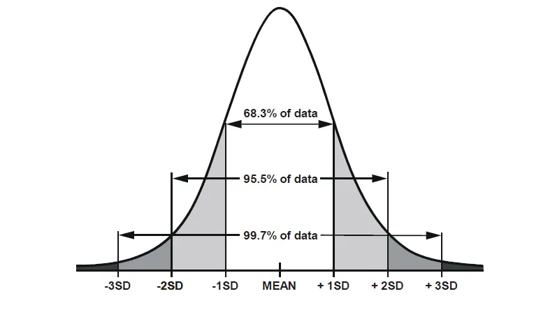
1st Standard Deviation includes 68.3% data spread from mean.
2nd Standard Deviation includes 95.5% data spread from mean.
3rd Standard Deviation includes 99.7% data spread from mean.
Low standard deviation = Near mean.
High standard deviation = Away from mean.
Residuals should be normally distributed, and distribution of errors should resemble a bell-shaped curve. This ensures that the errors have a symmetric distribution around zero For that, residuals should be independent from each other, meaning the residual of that observation should not be related to another observation. That’s why independence is crucial for accurate statistical prediction. We can draw the plot of residuals, and by doing so, we can see the flow of residuals. If there is no bell shape, then we can conclude there are outliers, and to find the outliers, we have many techniques, but one is the most commonly used, which is known as the interquartile range (IQR).
IQR is used to fix the ratio for detecting outliers, and once we get an outlier, we can manage it using various techniques
Q1 = data* 25%
Q2= data*50%
Q3= data*75%
IQR= Q3-Q1
Lower tail= Q1-1.5*IQR
Upper tail= Q3+1.5*IQR.
For finding extreme outliers:
Lower tail= Q1-3*IQR
Upper tail= Q3+3*IQR
Now below the lower tail and above the upper tail, whatever data we found these all we can consider as outliers.
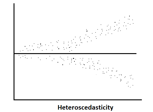
Homoscedasticity:
Whatever error the model gets after training, it should be constant with respect to the independent variable.
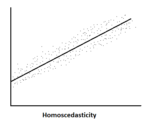
Homoscedasticity assumes that the scatter of the residuals is similar across the range of independent variables. That means spread of residuals should be constant for moderate, high, and poor predictors. The spread should be roughly the same across the range of predicted values If the homoscedasticity is violated, that means variability of the residuals changes as the values of the predicted values change; this is known as heteroscedasticity, and this spread may increase or decrease as the predicted values increase or decrease. And this leads to less precise parameter estimates, impacting the validity of statistical inference and making it difficult to accurately assess the significance of predictors.
Now let’s see some evaluation parameter of linear regression.
Residual / Error:
ε = y – ŷ
where:
ε: represents the residual.
y: represents the actual dependent value.
ŷ: represents the predicted value of the dependent value based on the regression model.
This is used to see the error between the actual and predicted values. Minimum residual is the key to an optimal model since models try to minimize errors by applying an inbuilt algorithm cum optimizer named “Gradient Descent Algorithm”.
Evaluation parameters are two types. If we are going to see only individual losses, then it is known as a loss function, and when we aggregate or average the individual losses over the entire training dataset, it is referred to as a Cost Function.
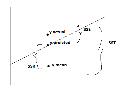
SSE (Sum of Squared Error):
It is the summation of the squared difference between the actual dependent values and the predicted dependent values.
SSE = Σ(yi – ŷi)²
- yi: represents the actual values of the dependent variable.
- ŷi: represents the predicted values of the dependent variable.
This is the summation of differences between the actual dependent and the predicted dependent values. By doing so, we can assume how our model is actually built. As I earlier said, the lowest error rate leads to an optimal model. But as we can see here, we are squaring the error rate. Why?
The answer is that when we build a model, some minor errors are ignored by model optimizer, which has an effect on the model’s performance. To avoid this, we take square of this error rate. In fact, we can say that model punishes the error rate by increasing its original value.
MSE (Mean Squared Error):
It is the summation of mean squared difference between the actual dependent values and the predicted dependent values.
MSE = Σ(yi – ŷi)²/n
- Where n is the number of data points.
MSE is used to take the summation of mean squared errors. MSE divides the error rate by the total number of observations, which gives us the normalized value of the error rate. Which is also known as a consistent estimator of the true error. MSE shows the average error made by the model. And due to normalization, it allows us to compare models with different numbers of data points. (SSE is not normalized since it is harder to compare models directly.)
MAE (Mean Absolute Error):
It is the summation of mean absolute difference between the actual dependent values and the predicted dependent values.
MAE = Σ(yi – ŷi)/n
At we seen in SSE, model punish errors to get focus, but sometimes the representation of big errors causes negligence at the smallest, tiniest error, and this is also not fair for any model. Even if error is small, it might create a very big problem in the model. So to avoid this, we use the absolute value of the error rate. One more reason is that large errors might be affected by outliers, and both SSE and MSE are outlier-sensitive, whereas MAE is not outlier-sensitive, and since we use MAE if there is an outlier present in the dataset,
RMSE (Root Mean Squared Error):
This is the summation of root-squared difference between the actual dependent values and predicted dependent values.
RMSE= sqrt (Σ(yi – ŷi)²/n)
Some time we need to use original units for errors. Whatever dependent value’s unit is there we need error rate also in same unit. For example suppose we are building a model where dependent variable’s measure is in dollars, then its error also we want to come in dollars. Which allowing direct understanding the problem or any important insights. It assessment the prediction accuracy to the scale of dependent variable. And for this we use Root Squared of Mean Squared Error.
SSR (Sum of Squared due to Regression):
This is the summation of squared difference between the predicted dependent values and the mean of the actual dependent values.
SSR = Σ(ŷi – ȳ)²
It is summation of squared difference between each predicted value and the dependent variable’s mean value. This measures the total variation in the predicted variable.
SST (Sum of Squared of Total Error):
This is the summation of squared difference between the actual dependent values and the mean of the actual dependent values.
SST = Σ(yi – ȳ)²
It is summation of the squared difference between total number of actual dependent value and the mean value of actual dependent variable.
This measure, total variation in dependent variable.
R2 Score:
It states how the model is built: a higher R2 score shows a well-built model, a lower R2 score shows a poor-built model.
R2 = 1 – (SSE / SST)
= SSE-SST/SST
- If SST> SSE: R2 Score will be +ve.
- If SSE>SST: R2 Score will be –ve.
R2 Score:
It is the main evaluation parameter in regression; by this parameter, we can conclude how our model is built. It states the goodness of our model. R2 scores measure the total proportion of variation in the dependent variable that is accounted by the independent variable. Indicating how models capture underlying relationships and patterns from data
- Score 0: State that the dependent variable has no variation. Which is a poor fit.
- Score 1: model explain all types of variation. It implies perfect fit and model will predict exact same dependent value. (But most of the time 1 indicates model overfitting, so we go for such value which is not actual 1, but near to 1, which indicating good fit.)
Limitation of R2 Score and overcomes by Adjustable R2 Score.
R2 Score tends to increase as predictors are added; even if the additional predictors do not improve the model performance, R2 score still slightly increases, which may cause overfitting. (Good on seen data, but bad on unseen data.) R2 score does not consider the number of predictors in the model; therefore, R2 score naturally increases, regardless of any actual contribution to the model. And also adding more predictors might create more complexity for the model.
To overcome this, we use its next updated version, named Adjustable R2 Score. By using this, we overcome the main limitation of the R2 score, which is, adjustable R2 score doesn’t increase as new predictors are added to the model, if that predictor is not going to make any positive contribution to model performance.
Adjustable R2 scores adjust the number of predictors in the model. It penalizes the inclusion of unnecessary predictors, providing a more reliable measure for model performance. This is addressed by accounting the model’s goodness and its complexity. It uses more meaningful comparisons between models with different numbers of predictors
Adjusted R2 = 1 – (1 – R2) * (n – 1) / (n – k – 1)
Where n is the number of dependent variables and k is the number of predictors in the model.
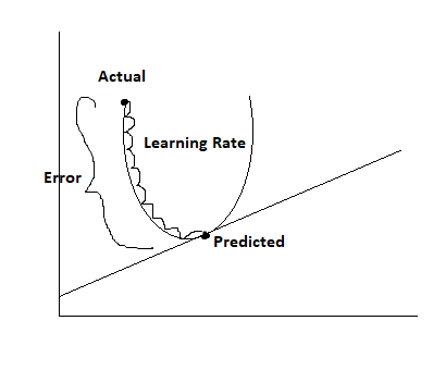
Gradient Descent:
Models have their own inbuilt algorithm named “Gradient Descent Algorithm,” which is also known as the optimizer for model. When the model takes out the errors, the next step is to minimize these errors and create an optimal model. To minimize the error, model use the gradient descent algorithm.
This algorithm is a parametric algorithm. Its parameter is learning rate, and by using this, this algorithm changes the model’s parameters values. Now the model’s changeable parameters are slope (m) and intercept (c). Because in the formula y=m*x+c, we cannot change the value of the input, so what remains is the slope and intercept value, and by updating this value in model, we try to minimize the error rate. The gradient descent algorithm uses partial derative to update the values of slope and intercept. Gradient descent updates this value on a global minima basis. Once the parameter value reaches the global minima or at the acceptance zone, it stops updating the values.
Formula:
new m= old m – learning rate* dy(cost function)/ dx(m)
new c= old c – learning rate* dy(cost function)/ dx(c).