StatusNeo

Exploring The Power of Predictive Modelling: Logistic Regression In Simple Word & In Depth.

Logistic regression is a type of supervised machine learning that uses labelled data. Logistic regression is used for classification. Logistic regression model, predict the probabilities of classes and choose one class whose probability is higher than others as a result or as an output of particular input data.

Logistic regression predicts the classes which is also known as categories since its labels should be in category format, and as usual, its predictors could be in continuous or categories. In multiclass classification, logistic regression works as one vs. the rest.

Even though it is known as a classification algorithm, we can still see that its name is logistic regression, a regression term used for predicting continuous values. But logistic regression predicts the probability for classification. How? The answer is that, at the back end of this algorithm, all operations are placed on the ground of regression, but only at the time of predicting the output, this model convert the regression values into class probability, and for that, it uses the logit odd function.

Formula: Sigmoid σ(y) = 1 / (1 + e^(-y))

= where,

y= m*x+c.

σ(y)=1 / 1 + e^- (m*x+c).

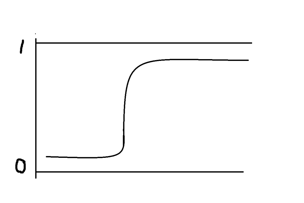
Logistic regression uses the S-shaped sigmoid curve to find the probabilities. This sigmoid curve lies between 0 and 1 range only, and therefore we can say that logistic regression is bounded between 0 and 1 range only for both binary and multiclass classification. And for classification between range 0 and 1 (in the sigmoid curve also, it is mentioned), model have a particular threshold value. By default, the threshold value is 0.5. Below 0.5, all data points lie in the 0th class, and above 0.5, all data points lie in the 1st class. And for multiclass classification, thresholds vary depending on the number of classes, but at the end, the model counts all classes probabilities and chooses the class with the highest probability as a result or output.

To find the probability, model use likelihood function. It is also known as maximum likelihood and estimation. The likelihood function use to count the proportion of that particular data point, which will use to decide which class to be considered for that particular data point. The likelihood always should be in positive but suppose model get negative likelihood that mean miss-classification is happening, then model will try to minimize that negative likelihood proportion, by which model make assure itself for true classification. 

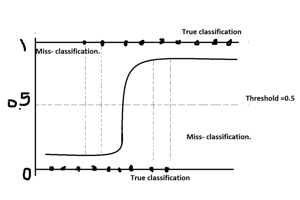
In logistic regression, the model draws an “S-shaped sigmoid curve. In the below figure, you can see what is an S-shaped curve is, what is threshold, what is boundary, what miss-classification is, and what true classification.

let’s understand this, by a simple table:

Class	Age	Diabetes	Model prediction
0	20	N	T
0	30	N	N
0	40	N	N
1	50	T	T
1	60	T	T
1	70	T	N
1	80	T	N

in above table, you can see there is three model prediction goes wrong, that mean they are actually different but model predict different, for example at age of 20 that person doesn’t has the diabetes but model predict he has, and below whose age is 70 and 80 they both have diabetes actually but model predict they both doesn’t have diabetes. This is called miss classification, which means if there is something in the actual and the model predicts something else that does not relate to their class, then that is known as miss classification.

Sigmoid Function:

It is a mathematical function that is used to map the predicted value to determine the probability of a class. It maps the value in the range of 0 to 1, which will never go beyond this limit. since the Sigmoid’s shape is fixed as an “S” shape.

Now before we go in depth on how logistic regression actually works, let’s see what actually probability is.

Probability is nothing but a numerical representation of the likelihood of an event.

1. Numerical
2. Likelihood
3. Events

Numerical:

Comes directly in numerical format like 0 or 1.

Likelihood:

More closer to 0 means more likelihood to 0^th class.

More closer to 1 means more likelihood to 1^st class.

————————————————————————————————————————————————————————————————-

For example:

—————————————————————————————————————————————————————————————————-

• Probability of one particular input is 0.9 then. And it lies in class 1^st .
• Mathematically we can find it by subtracting its opposite class number from that input’s probability.
• 0 – 0.9 = 0.9
• This 0.9 answer show that, the input is egger to join 1^st  class and its eagerness shows probability of 0.9 out of 1. This mean 90% of eagerness to join class 1^st .

—————————————————————————————————————————————————————————————————-

• Probability of one particular input is 0.6 and input lies in class 1^st .
• Mathematically we can find it by subtracting its opposite class number from that input’s probability.
• 0 – 0.6 = 0.6
• This 0.6 answer is more than the default threshold of 0.5, and since that input is eager to join 1^st  class, we can conclude that 

—————————————————————————————————————————————————————————————————-

Events:

Events is nothing but outcomes of experiments.

For example: suppose we are going to find the probability of a coin; then, it will count on basis of events and samples.

                             P= n(events)/n(samples).

For Example let’s take coin.

• Events: in coin there is 1 possibilities of event, which we are going to choose, either head or tail.
• Samples: samples are 2 possibilities of coin while tossing; head and tail.

Now, suppose we want to calculate the probability of head while tossing a coin then.

=n(events)/n(samples)

=½ =0.5

If a coin tossed, there is a 0.5% chances, that it will land on its head.

Similar for dice.

Events is 1.

Samples is 6.

To find the probabilities of any event:

1/6=0.16

                             In dice, the probability of an event is 0.16%.

How does the sigmoid work, or how does the probability convert the continuous value?

We know that at the back end, all operations are placed on the ground of linear regression, and their results come in the range (-∞, +∞), but at the time of the result, the result should be in the range 0 to 1. And for that model, use the logit odd function. Which is nothing but the inverse of the sigmoid function.

RHS(-∞, +∞) = LHS (0, 1)

=we know log(0) = -∞

=for converting +∞ we use Odds.

          Odds(A) = p / (1 – p)

=so now equation will be:  log(0,odds)

This equation convert the (-∞, +∞) in to range 0 to 1.

Assumption in logistic regression.

• For binary classification, it require dependent variable should be in two categories, and for multiclass dependent variable should be more than two categories.

• Logistic regression require, target variable should be independent with each other. That means target variables shouldn’t come from repeated measurements.

• Logistic regression require, no multicollinearity between independent variable. Here because of limited boundaries, there is might be possibilities of near about similar independent values found. But there shouldn’t be high correlation in between independent variables.

• Logistic regression require linearity between independent variables and log odds

• Logistic regression require large sample size.

Evaluation Parameters:

Once model built, we go for evaluation for find out how the actually model is built, is it god fit or poor fit.

Log –Loss function:

Log loss is an indicator of how close the prediction probability is to the corresponding actual value.

Log-Loss (ya, yp) = -(1/n) * Σ [ ya * log(yp) + (1 – ya) * log(1 – yp) ]

Where:

• “ya”=  it is the actual binary labels (0 or 1)  in the dataset.
• “yp”= it is the predicted probabilities of classes.
• In the formula, “n” represents the number of instances in the dataset, and Σ denotes the sum of all instances.
• ya * log(yp): This term is activated when the actual label (ya) is 1. It measures the log-likelihood of the predicted probability for the positive class being correct.
• (1 – ya) * log(1 – yp): This term is activated when the actual label (ya) is 0. It measures the log-likelihood of the predicted probability for the negative class (1 – yp) being correct.

Let’s understand this by simple example:

• yp = [0.8, 0.3, 0.6, 0.9]
• ya = [1, 0, 1, 1]
• To calculate the log loss for this example, we’ll use the formula: log_loss(ya, yp) = -(1/n) * Σ [ ya * log(yp) + (1 – ya) * log(1 – yp) ]
• where “n” is the number of instances (in this case, n = 4), and Σ denotes the summation over all instances.
• Now, let’s calculate the log loss step by step:

So, in this example, the log loss for the given predicted probabilities and true actual labels is approximately 0.299. Lower values of log loss indicate better model performance, as it means the predicted probabilities are closer to the actual labels. And if the model finds a higher loss, then automatically the model’s inbuilt algorithm, cum optimizer, comes into play, which is named the Gradient Descent algorithm, which helps reduce the log loss by applying the partial derivative and learning rate parameter.

Confusion Matrix:

          Confusion matrix is a matrix which shows how many data points are truly classified and how many are misclassified. It is 2*2 matrix if there is binary classification, and it is n*n matrix if there is multiclass classification, whether n is the number of classes.

Figure:

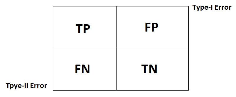
In above figure you can see four main parameters, named TF, TN, FP, FN.

TP (True Positive): Actually positive class and the model also predicted positive class.

TN (True Negative): Actually negative class and the model also predicted negative class.

FP (False Positive): Actually negative class but the model predict positive class.

FN (False Negative): Actually positive class but the model predict negative class. 

We can find each classification ratio. Let’s look over there:

Suppose there is 50 data points and among them distribution as follows:

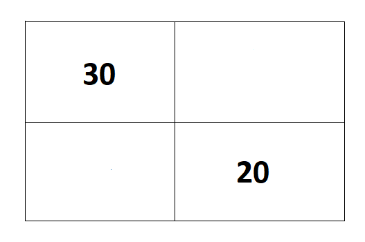
True 30 and negative 20.

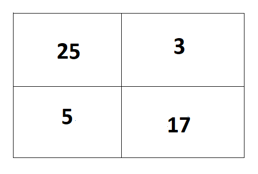
But model prediction is: TP= 25,

                                                TN=17,

                                                FP=3

                                                FN=5

TPR (True Positive Ratio):

                   TP/(TP+FN) = 25/30

                                      = 0.83%

—————————————————————————————————————————————————————————————————-

TPR is also known as Precision.

FPR (False Positive Ratio):

                   FP/(FP+TN)= 3/20

                                      =0.15%

—————————————————————————————————————————————————————————————————-

FNR (False Negative Ratio):

                   FN/(FN+TP) = 5/30

                                      =0.16%

FNR is also known as Recall.

—————————————————————————————————————————————————————————————————-

TNR (True Negative Ratio):

                   TN/(TN+FP) = 17/20

                                      =0.85%

—————————————————————————————————————————————————————————————————-

What is Precision and Recall?

Precision: It is ratio of model predicted positive values with respect to actual positive values.

Recall: It is ratio of model’s falsely predicted values as negative with respect to actual positive values.

This both are very crucial, because as per nature of model, this will vary. Let’s understand this with real time example.

Precision:

          In a stock market prediction model, the model gives information about when the market is going to collapse and when it is not. (Market collapse = 0th class, and market collapse is not 1st class.) Now suppose the market is going to collapse, but the model says the market is not going to collapse. This is a miss-classification because, actually, it should be positive but the model predicts it as negative. And suppose, on the basis of the model, if the user stayed relaxed, he might face a huge loss. Since we need such a model that tries to classify accurately, Since precision is important, the model focuses on increasing the highest precision rate. The highest true classification is a solution to increase the precision rate.

Recall:

          Suppose we have one model that is predicting whether the mail is spam or not (spam = 0th class and not spam = 1st class). Now suppose one mail is genuine but the model predicts it as Spam, so there might be a possibility of losing genuine mail. Here, actually, the mail is genuine, but model classifies it as spam, which means model prediction is miss-classified.

The model always tries to increase the precision and decrease the recall; to decrease the recall, the model should increase true positive prediction and increase the precision at the cost of a lower recall.

Accuracy Score:

                   TP+TN/ (TP+TN+FP+FN)

It is a proportion of correct predictions over total predictions; this is important until we have a well-balanced data set. Suppose we get data that is not well-balanced; then its accuracy is totally biased. How?

Let’s assume one dataset is there, where 0th-class data is in 90% and 1st-class data is in 10% of the total dataset. Now suppose the model predicted 90% accuracy. But due to the imbalanced dataset, whatever accuracy model is giving is totally inverse, which means its accuracy is actually 10%, which is not good. Now, to avoid such problems, we need to focus on precision and recall, and the F1 score is an evaluation parameter that uses this precision and recall to conclude the model’s accuracy.

F1 Score :

The F1 score is nothing but the harmonic mean of precision and recall.

F1_score= 2* (precision*recall) / (precision+ recall).

In F1, precision and recall have equal weight. Accuracy scores only measure the percentage of corrected classified predictions that are model-made.