The gradient descent algorithm is an optimization algorithm, that is commonly used to train machine learning models and neural networks. This algorithm helps the model learn the pattern of the given data in the training phase. Models use the cost function as a barometer, which should decrease with each iteration, and with each iteration, the gradient updates the coefficient value, until the error rate becomes minimal or equal to zero.
Machine learning with the gradient descent algorithm emerges as a powerful model in AI.
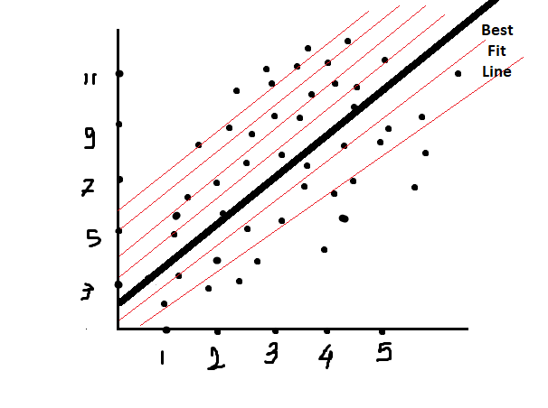
Before diving into gradient descent, we need to just memorize some parts of linear regression. In Linear Regression, the model draws multiple fitted lines that travel between data points. And assume one line as the best-fit line that covers the maximum number of data points while traveling.
.
In the next below image, we can see that some points are away from the linear line. As we know that the best-fit line travels from such an area, the maximum number of data points should be covered. But it doesn’t mean that all data points will lie on a linear line. We didn’t come across such data; even if do, it will be pure linear data, and it is not difficult to work on such data; just apply the algorithm, take inputs for testing, and give the result. Since the data is pure linear here, the model will directly compare the range of the result and answer in that range. But actually, this is not going to happen; we didn’t get such data, and even the best data we found will not cross the linearity threshold by more than 80%.
Modeling on such data will not produce a good fit; to make a good fit, we need to make the data linear. Even though we cannot change the original data structure, we can make minor changes that aid in model fit. Now the question arises: who will do this? The answer is the gradient descent algorithm. But how? By updating the coefficient values.
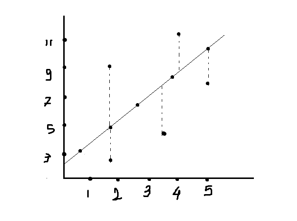
In the above figure, some data points are away from the linear line. These data points are trying to jump on a linear line by updating the values of coefficients. The difference between two points is nothing but the distance, and this distance is measured in the form of error or residual. This distance has never been in minus, but somewhere we say positive distance and negative distance.
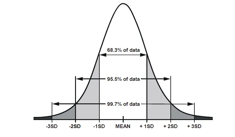
Gradient descent Try to make this distance rate equal to 0 or minimal, but note that the model only succeeds with those data points that are within the 3rd standard deviation range. Because, as we know, up to the 3rd standard deviation, all data is assumed to be data, and after the 3rd standard deviation, data points are assumed to be outliers.
Let’s play a simple game: suppose there is one boy whose role is to throw the ball in the basket from some specific distance
1.In his first attempt, he threw the ball, but it didn’t reach the basket; instead, it landed before the basket
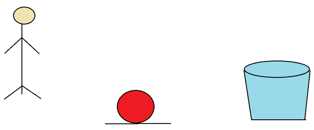
Now what happened here, is that the force or power to throw the ball was not sufficient since the ball did not reach its destination
2. In his second attempt, he threw the ball, but this time also it didn’t reach its destination; instead, it covered some maximum distance and landed after the basket.
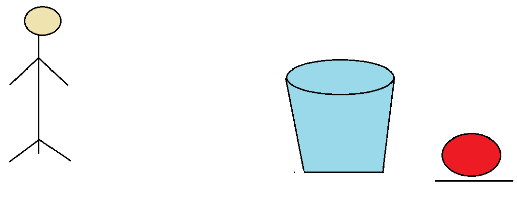
What happened here, was at last time he missed the basket because of less power, but now he adds some extra power and throws the ball toward the basket. But in this step too, he didn’t get success. Because of some unnecessary extra power, the ball landed after the bucket.
3. In the third step, the boy throws the ball and, yes! The ball reaches its proper destination, which is in the bucket
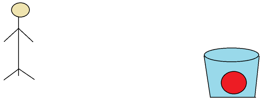
In his third attempt, he applied not the minimum and not the maximum power; instead, he applied the appropriate power. And he gets the result that he wants.
You will now ask, what is the relation between this game and the gradient descent algorithm? The same phenomenon is used in gradient descent to reduce the error rates and update the appropriate value of coefficients until the error rate is minimal or equal to zero.
Gradient descent is a parametric algorithm, which is a learning rate. Using the learning rate model, update the values of the coefficients of the model. This process is known as the learning of models. In this process, models learn the patterns of data, and this learning helps to make decisions. The learning rate is a very small value. Due to its very small value, it is also known as a baby step, which applies in mathematical equations and takes out the new coefficient’s value. The learning rate’s value is 0.001.
—————————————————————————————————————————————————————————————————-
Gradient descent uses the partial derivative. The formula of gradient descent is:
New_m = Old_m – learning_rate * (d(MSE) / d(m))
New_c = Old_c – learning_rate * (d(MSE) / d(c))
- New m= new value for coefficients slope ‘m’
- old m= old value of coefficients slope ‘m’
- New c= new value for coefficients intercept ‘c’
- old c= old value for coefficients intercept ‘c’
- d(MSE) / d(m)= derivative of cost function with respect to slope
- d(MSE) / d(c)= derivative of cost function with respect to intercept
—————————————————————————————————————————————————————————————————-
Now let’s take one simple dataset:
x = [2, 4] # Input feature
y = [3, 6] # Target values
m = 0.5
c = 1.0
Learning rate = 0.01
Iteration:1
Step 1:
Compute the current value of MSE using the initial “m” and “c”:
MSE: ∑ i=1 n(y_actual –y_predicted)^2
Y_predicted= m*x+c
Step 2:
Compute the current value of MSE using the initial “m” and “c”:
MSE=1/2[(3−(0.5×2.4+1))^2+(6−(0.5×2.4+1))^2]≈1.5036
Step 3:
Calculate the gradients of MSE with respect to “m” and “c”:
d(MSE)/d(m)= ½ [ −2 × 2.4 × (3 − (0.5 × 2.4 + 1 )) −2 × 2.4 × (6 − (0.5 × 2.4 + 1 ))] ≈ −3.600
d(MSE)/d(c)=
½ [ −2 × (3 − (0.5 × 2.4 +1 )) −2 × (6 −(0.5 × 2.4 + 1))] ≈ −1.800
Step 5:
Update the values of “m” and “c” using the gradient descent update rule:
New_m = 0.5 – 0.01 * (-3.600) ≈ 0.536
New_c = 1.0 – 0.01 * (-1.800) ≈ 1.018
—————————————————————————————————————————————————————————————————-
Iteration:2
Calculate the gradient of MSE with respect to updated m and updated c:
MSE ≈ 1.1708
d(MSE)/d(m) ≈ -2.630
d(MSE)/d(c) ≈ -1.311
By this value new updated value of m and c:
New_m = 0.5 – 0.01 * (-2.630) ≈ 0.5636
New_c = 1.0 – 0.01 * (-1.311) ≈ 1.0315
—————————————————————————————————————————————————————————————————-
Iteration:3
Calculate the gradient of MSE with respect to updated m and updated c:
MSE ≈ 0.9121
d(MSE)/d(m) ≈ -1.8472
d(MSE)/d(c) ≈ -0.9236
By this value new updated value of m and c:
New_m = 0.5 – 0.01 * (-2.630) ≈ 0.5819
New_c = 1.0 – 0.01 * (-1.311) ≈ 1.0404
—————————————————————————————————————————————————————————————————-
Iteration:4
Calculate the gradient of MSE with respect to updated m and updated c:
MSE ≈ 0.7320
d(MSE)/d(m) ≈ -1.3032
d(MSE)/d(c) ≈ -0.6516
By this value new updated value of m and c:
New_m = 0.5 – 0.01 * (-2.630) ≈ 0.5949
New_c = 1.0 – 0.01 * (-1.311) ≈ 1.0479
—————————————————————————————————————————————————————————————————-
Iteration:5
Calculate the gradient of MSE with respect to updated m and updated c:
MSE ≈ 0.5863
d(MSE)/d(m) ≈ -0.9232
d(MSE)/d(c) ≈ -0.4616
By this value new updated value of m and c:
New_m = 0.5 – 0.01 * (-2.630) ≈ 0.6042
New_c = 1.0 – 0.01 * (-1.311) ≈ 1.0515
—————————————————————————————————————————————————————————————————-
We continue this process until the MSE converges to a minimum or until a predefined number of iterations is reached. The values of “m” and “c” obtained after convergence will represent the best-fitting line that minimizes the MSE for the given dataset.
We have two types of gradients:
- Negative Gradient
- Positive Gradient
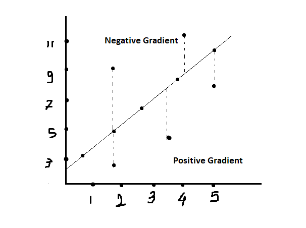
Negative Gradient:
If a data point lies above the linear line, it means the predicted value (on the line) is less than the actual value. In this scenario, the loss function may increase (assuming squared error loss), which would lead to a negative gradient. The algorithm then uses this negative gradient to update the parameters in the direction that reduces the loss, aiming to bring the predicted value closer to the actual value.
Positive Gradient:
If a data point lies below the linear line, it means the predicted value (on the line) is greater than the actual value. The loss function may increase in this case as well, leading to a positive gradient. The algorithm then uses this positive gradient to update the parameters in the direction that reduces the loss, bringing the predicted value closer to the actual value.
Learning rate:
Why learning rate is 0.001?
What if we use a too-small learning rate?
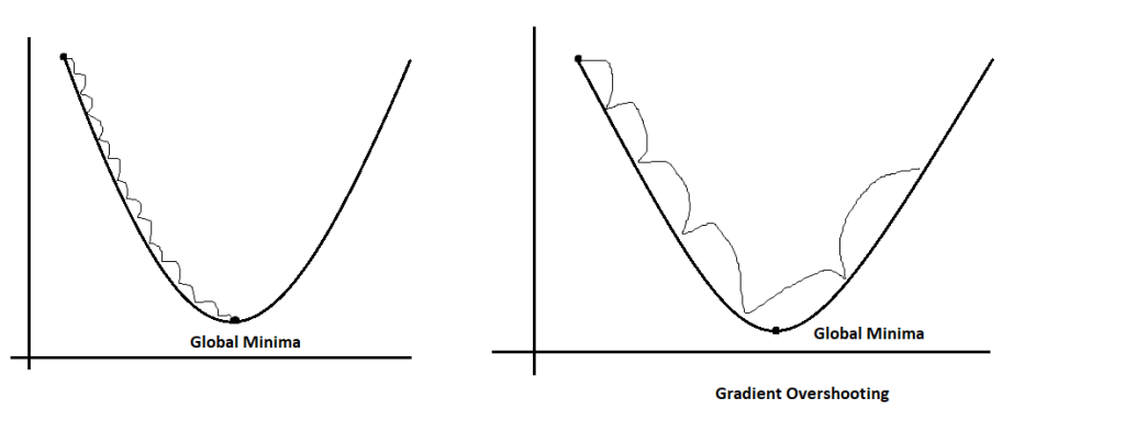
Memorize the above ball and basket game; if the learning rate is too small, we face the gradient vanishing problem. Like in his first attempt, the boy couldn’t achieve success, and the ball fell before the basket. Similarly, gradients can’t reach a particular destination, which is known as the global minima. Instead of that, it stuck at the local minima.
Suppose we have an old value of slope ‘m’ = 5, and after applying the derivative, the model updates the value to the new slope ‘m’, which is 4.999999. Now we can see that there is not any noticeable new value. It just decreased by 0.000001, which means the update was stuck at that point. This is known as gradient vanishing.
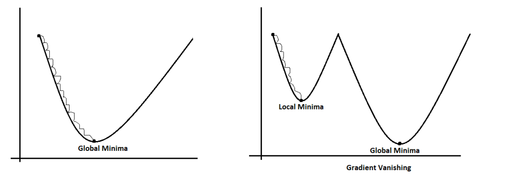
What if we use big values as learning rates?
Again, move to the example of the ball and basket game; here, at the second attempt, when the boy increased his power and throws, the ball fell after the basket. That means if you apply more power than required, it will go away from your destination. Similarly, if there is a large learning rate, one might face the gradient overshooting issue, where gradients sometimes increase and sometimes decrease, and in this cycle, there might be possibilities of losing global minima.