K-Nearest Neighbor is a type of supervised machine learning that is used for both regression and classification. It is a non-parametric algorithm, which means that in this algorithm, we don’t have any assumptions. K-NN finds the similarities between data points by calculating the distance among them, since it is also known as a distance-based algorithm. Based on this calculation of distance, if there is a classification problem, then using voting, the model finds the probability of class. If there is a regression-related problem, then the model finds neighbor’s mean. This mean is produced as a result of regression-related input.
It is also known as a lazy learner, because this algorithm just saves the training data as it is in memory, not performing any operations on it while training. But when the model gets new input (the test case) for prediction, then the model starts the actual operation. The model is going to find the distance between each data point and input and compare all distance calculations to find out which are more similar and which are too close to each other. All operations are heavily time-consuming since the model is known as a lazy learner, which means training is very fast but testing is time-consuming.
How does it work?
K-Nearest Neighbor’s name itself gives a hint about the working strategy. This algorithm finds the closest data points based on inputs. Now how many neighbors are needed to compare for predicting the result is decided by the “K” value. K is nothing but the number of neighbors; how much k value we give that much neighbors is going to select, and those are should be more closely input data point. Suppose K = 5, which we have taken, and then the algorithm finds 5 too-close neighbors that are near that input data point in the distance. Now, once you have selected the top 5 neighbors, find out the majority between neighbors in the case of classification or the mean in the case of regression. This majority, or mean, is the result of that input data point.
Let’s understand it by image:
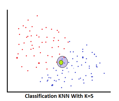
- Classification: neighbors found like (0, 1, 0, 1, 1)
Where,
- Class 0
- Class 1
—————————————————————————————————————————————————————————————————-
Now we know that in classification, using a voting model predicts the result class. As per this condition, the above neighbors
0th class — comes 2 times,
1st class –comes 3 times.
And from voting at the last model, choose 1st class as the result.
————————————————————————————————————————————————————————————————-
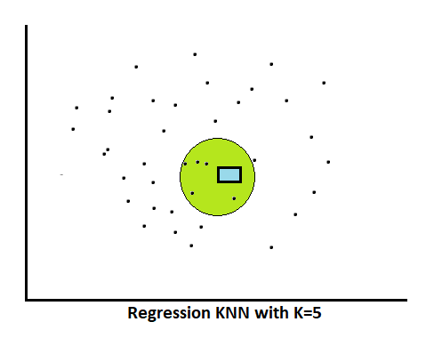
Regression: neighbors found like (40000, 37000, 28000, 35000, 30000)
As we know, in regression, the model counts the neighbor’s mean and uses this mean value as the output for the test case.
(40000 + 37000 + 28000 + 35000 + 30000) / 5 = 34000
The answer will be 34000.
—————————————————————————————————————————————————————————————————-
The K value should be at least above 5. The default value of k is 5, but we can increase and decrease it.
Why we should give a K value above 5?
Noise Increase: If we use a smaller k value, less than 5, then the algorithm might find noise and outliers in the dat, because a smaller number of neighbors may be heavily affected by those data points which might not be representative of the overall pattern in the data.
Overfitting Increase: If we give a very small k value, or less than 5, it tends to increase the risk of overfitting, especially if the dataset is noisy or has a lot of outliers. Overfitting occurs when the model fits the training data too efficiently rather than generalizing well to unseen data.
Variance Increase: If we give a very small k value, less than 5, this leads to a higher variance in the predictions. Because different neighbors might lead to different results. This could result in less stability in the model.
Create Complex Decision Boundaries: If we give a very small k value, or less than 5, it results in more complex decision boundaries, which might lead to miss-segmentation and loss of data.
Computationally Fast: If we give a very small k value, or less than 5, it make the algorithm computationally faster. Because it involves fewer neighbors to be considered for each prediction. But in the end, this model will not be built as a good-fit model or an optimal prediction model.
Now what happens if the model uses an even number as a “K” value and a tie happens in voting while classification? Then there are two methods that generally follow:
- Count the number of data points in each class, and put that class as the result of which class has more data points.
- If a tie happened in the above condition also (that means data points are equal in both classes), then go with the principal rule. Select the first class, which will be the 0th.
The distance model has two criteria:
- Manhattan Distance
- Euclidean Distance
These parameter’s “p” values are 1 and 2, respectively. This “p” value is used by the model to select which criterion to use to calculate the distance.
Both criteria are derived from the Minkowski principle.
Minkowski distance = ( Σ ( |xi – yi |p ) ) 1/p.
Where,
When p = 1, it gives the Manhattan distance (L1 distance).
When p = 2, it gives the Euclidean distance (L2 distance).
—————————————————————————————————————————————————————————————————-
Euclidean:
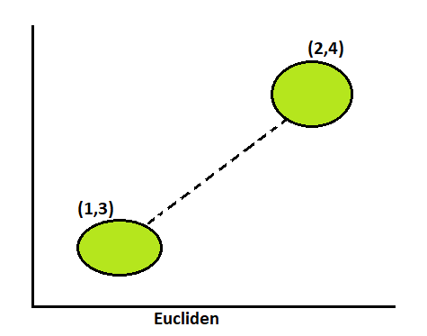
This distance parameter counts the distance from point to point.
Formula of Euclidean = ((x2 – x1)2 + (y2 – y1)2)
As earlier said, it is derived from Minkowski. Let’s see how. As we know, the “p” value of Euclidean is 2. Use these two values in the Minkowski formula, and we get the Euclidean formula.
Euclidean distance When p = 2
Minkowski distance = ( Σ ( |xi – yi |p ) ) 1/p.
= (Σ ( |xi – yi|2 ) ) 1/2
= √ ( Σ ( |xi – yi|2 ) )
Step 1: Write down the coordinates of the two points.
Point 1: (2, 3)
Point 2: (5, 6)
Step 2: Calculate the differences between the corresponding coordinates (x and y) of the two points.
The difference in x-coordinates is 5 – 2 = 3.
The difference in y-coordinates is 6 – 3 = 3.
Step 3: Calculate the squared differences for the Euclidean distance.
The squared difference in x-coordinates is: (3)2 = 9.
The squared difference in y-coordinates is: (3)2 = 9.
Step 4: Sum up the squared differences.
The sum of squared differences is 9 + 9 = 18.
Step 5: For the Euclidean distance, take the square root of the sum of squared differences.
Euclidean distance = 18 ≈ 4.24 (rounded to two decimal places)
—————————————————————————————————————————————————————————————————-
Manhattan:
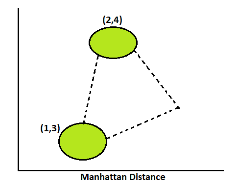
The Manhattan distance technique counts the distance by adjacent sides. And its result is always greater than Euclidean, since priority gives Euclidean.
Manhattan Formula: Σ ( |xi – yi |p )
As earlier said, it is derived from Minkowski. Let’s see how. As we know, the “p” value of Manhattan is 1. Use this 1 value in the Minkowski formula, and we get the Euclidean formula.
Euclidean distance When p = 2:
Minkowski distance = ( Σ ( |xi – yi |p ) ) 1/p.
= (Σ ( |xi – yi |1 ) ) 1/1
= Σ ( |xi – yi |)
Step 1: Write down the coordinates of the two points.
Point 1: (2, 3)
Point 2: (5, 6)
Step 2: Calculate the differences between the corresponding coordinates (x and y) of the two points.
The difference in x-coordinates is 5 – 2 = 3.
The difference in y-coordinates is 6 – 3 = 3.
Step 3: Calculate the absolute differences for the Manhattan distance.
Absolute difference in x-coordinates: |5 – 2| = 3
Absolute difference in y-coordinates: |6 – 3| = 3
Step 4: Sum up the absolute differences.
Manhattan distance = 3 + 3 = 6.
Manhattan distance between Point 1 and Point 2 = 6.
—————————————————————————————————————————————————————————————————-
Because of the distance-based algorithm, we need to scale down the data set to avoid biased results. We have two popular scaling features:
- Min-Max Scalar (Normalization)
- Standard Scaler (Standardization)
Why scaling? Because of distance-based algorithms, distance is going to count between data points; if one variable’s count is in the thousands and another variable’s count is in the hundreds, this difference is going to affect the results since scaling is compulsory in all distance-based algorithms.
Advantages of KNN:
- It is a non-parametric algorithm (No assumptions).
- It is useful for both classification and regression, but mostly for classification.
- We don’t have a training step here, so it is much faster than any other algorithm.
- Easy to implement
- Convert the multiclass classification to a binary classification.
- Only two hyperparameters are there: “p-value” and “K value”.
Disadvantages of KNN:
- Lazy learner (Testing is heavily time-consuming)
- It is a Distance-based algorithm, since we need feature scaling,
- Each time, we have to find the best “k” and “p” values.
- Sensitive to outliers
- Get affected if there is an imbalanced dataset.
- Cannot be used with high-dimensional datasets because of lazy learning.