StatusNeo

OPTIMIZATION: A Pillar of Machine Learning

Do you know how Netflix recommend you a movie based on your past views? How your spam emails are directly diverted to the spam section of your email? How you are able to search something using voice search? Do you know how does Optimization works in these applications of Machine Learning?

There are many queries like this which can be answered by the term Machine Learning. Now let’s see what does Machine Learning means?

Machine Learning is the science (and art) of programming computers so they can learn from data.

Let’s understand it with the help of an example. In humans when a baby is born, we teach them the basics of living a life over a period of time like what to eat, how to speak in native language etc based on the teachings the child behaves and act accordingly. Similarly, Machine Learning is method of teaching machines (Computers) how to react by programming them such that they can learn from data and provide insights accordingly

PILLARS OF MACHINE LEARNING

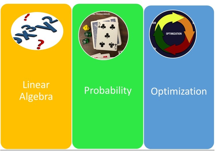
There are mainly three pillars on which Machine Learning Algorithms operate.

1. Linear Algebra : Linear Algebra helps us to understand the structure and relationship between data which machines use to learn from.
2. Probability: Probability is used to deal with the Noise and uncertainty in data. Noise is basically the error recorded during measuring or collecting data.
3. Optimization: Optimization is a mathematical tool that allows us to convert data to decisions.

INTRODUCTION TO OPTIMIZATION

When we train our model with the data, we care about finding the best results. Optimization helps us in finding the best results which can be used as decisions derived from the data.

Why do we optimize our machine learning models? We compare the results in every iteration by changing the hyperparameters in each step until we reach the optimum results. We create an accurate model with less error rate.

The two main goals of Optimization is following:

• Maximising Rewards
• Minimising Loss

Let’s see the general form of equation we use to solve a problem to get best results using optimization.

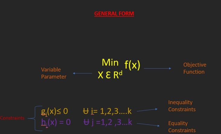
• Objective Function: The Objective function is a mathematical optimization problem equation which can be either minimized or maximized.
• Constraints : Constraints are logical conditions that a solution to an optimization problem must satisfy. It limits the capacity of the objective function.

BASIC ALGORITHM FOR UNCONSTARINED OPTIMIZATION : GRADIENT DESCENT

Whenever there is no logical condition or limit to the input of an optimization problem then we call it as Unconstrained Optimization.

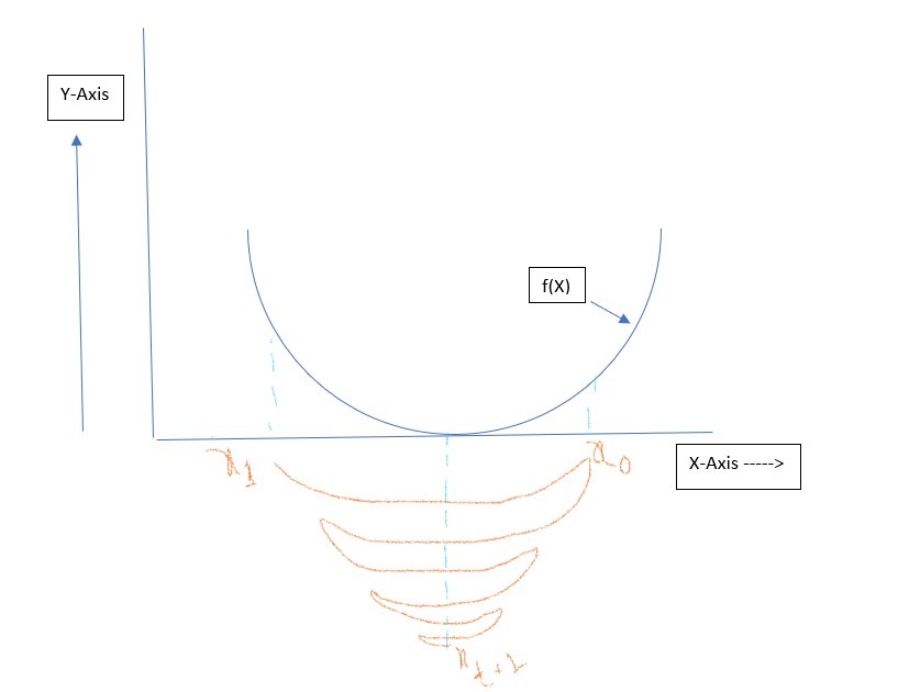
For example suppose X_t is first input for the Objective Function. Based on the output we get we try to move either right direction or left direction of X_t  on X-axis to find an optimal solution. Let’s suppose the next input value would be X_t+1.We do this iteratively till we find an optimal value for X which gives us minimum error in our Objective function. One important observation in the graph is that the slope changes its sign from positive to negative at minima. As we move closer to the minima, the slope reduces.

Now,

X_t+1 = X_t – ŋ f `( X_t)

Where,

ŋ  = learning rate (also called Step Size)

f `( Xt) = first derivative of f(X).

Gradient Descent : Gradient Descent is a very generic optimization algorithm capable of finding optimal solution to a wide range of problems.

X_t+1 = X_t – ŋ f `( X_t)

Where,

ŋ  = learning rate (also called Step Size)

f `( Xt) = first derivative of f(X).

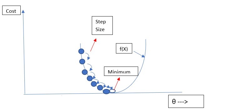
Gradient Descent measures the local gradient of the error function with regards to the parameter vector θ, and it goes in the direction of descending gradient. Once the gradient is zero, you have reached a minimum. Gradient Descent converges to local minimum.

For Convex Functions local minimum is also global minimum. Gradient Descent algorithm is good fit for convex function to find global minimum.

Stochastic Gradient Descent : Stochastic Gradient Descent just picks a random instance in training set at every step and computes the gradients based only on that single instance. Obviously this makes the algorithm much faster since it has very little data to manipulate at every iteration.

What is Learning rate?

An important parameter in Gradient Descent is the size of the steps, determined by the learning rate hyperparameter. If the learning rate is too small, then the algorithm will have to go through many iterations to converge, which will take long time. On the other hand, if the learning rate is too high, you might jump across valley and end up on the other side, possibly even higher up than you were before.

CONSTRAINED OPTIMIZATION

The Real-life problems comes with different types of constraints. Optimizing these constraints setup would provide an approximation which would be as close as possible to the actual solution of the problem, but would also be feasible.

Descent direction : A direction that reduces the Objective function f(x) value, d^T∇f(x)<0.

Feasible direction : A direction that takes to a point satisfying constraint function g(x)≤0.

Suppose we have an Objective function named f(x) such that x Ɛ R^d  and constraint g(x)≤0. Now to find an optimal point x*

1. g(x*)≤0
2. No descent direction is a feasible direction.

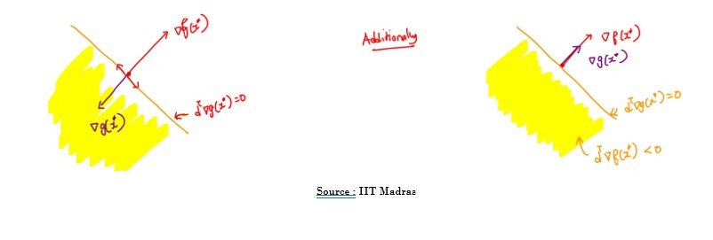
So, the necessary condition for optimality at a point x* is  d^T∇g(x*)=0.

And Optimal Configuration :

∇f(x*)=-λ∇g(x*) 

where λ is a positive Scalar Value.

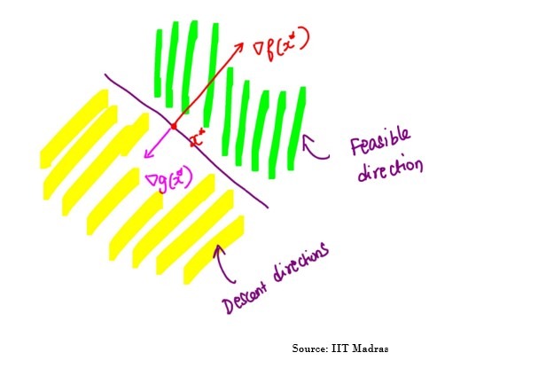
As per IMG 6, Feasible and descent direction are anti-parallel to each other.

METHOD OF LAGRANGE MULTIPLIER

Lagrange Multiplier is a method in optimization which is used to find Local Maxima or Minima of a Objective function subject to a equality constraint.

Suppose we have an Objective function named f(x) such that x Ɛ R^d  and constraint g(x)=0.

So, the necessary condition for optimality at a point x* is  d^T∇g(x*)=0.

And Optimal Configuration :

∇f(x*)=λ∇g(x*) 

where λ is any arbitrary Value(positive or negative) known as Lagrange Multiplier.

Other Fast Optimizers

• Momentum Optimization
• Nesterov Accelerated Gradient
• AdaGrad
• RMSProp
• Adam Optimizaton
• Learning Rate Scheduling

Conclusion

In the above article we learned about the Constrained and Unconstrained Optimization technique which is quite helpful in solving a real life problem on data. Optimization helps us to be as precise as we can in predicting the outcome based on data. Optimization has wide range of application in deep neural network which helps to enhance the performance of a machine Learning model.