Efficient Opti: Mastering Stochastic Gradient Descent
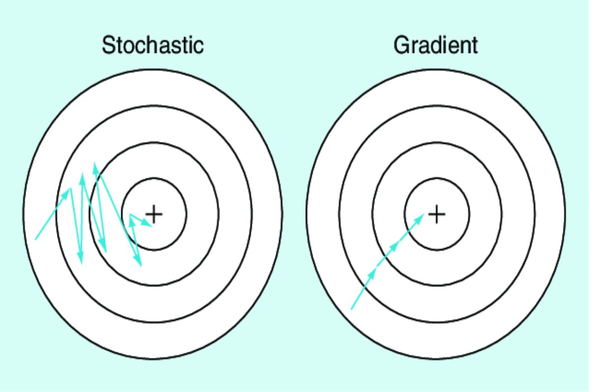
Stochastic Gradient Descent (SGD) is a variant of the Gradient Descent optimization algorithm. While regular Gradient Descent computes the gradient of the entire dataset to update model parameters, SGD updates the parameters using the gradient computed from a single randomly chosen data point (or a small subset of data points) in each iteration. This introduces randomness into the optimization process and can lead to faster convergence, especially in large datasets
Features of Stochastic Gradient Descent:
Randomness:
- The key characteristic of SGD is introducing randomness by processing one data point at a time. This randomness can lead to noisy updates but also helps escape local minima.
- SGD processes one data point (or a small batch of data points) at a time to update the model’s parameters. This introduces randomness because the choice of which data point to use at each step is random.
- The randomness in SGD leads to noisy updates. Since each data point is randomly chosen, the gradient computed for that data point may not represent the “true” gradient of the entire dataset
- While noisy updates can seem like a disadvantage, they can be beneficial. In non-convex optimization problems (common in deep learning), there may be many local minima in the cost function. Deterministic optimization methods like Gradient Descent are more likely to get stuck in these local minima. The randomness in SGD allows it to occasionally jump out of local minima and explore other regions of the parameter space.
- The noisy updates in SGD allow it to converge faster compared to batch Gradient Descent in many cases. This is because it escapes local minima more easily and explores a broader range of parameter values.
- The amount of noise in SGD is controlled by the learning rate. A higher learning rate introduces more randomness and larger updates, which can make the optimization process more erratic. A smaller learning rate reduces the randomness but might slow down convergence. Choosing an appropriate learning rate is crucial in SGD.
- By introducing randomness, SGD can reduce overfitting. Overfitting occurs when a model learns the noise in the training data, rather than the underlying patterns. The noisy updates in SGD can help prevent the model from fitting the training data too closely
Faster Convergence:
- SGD’s frequent updates can lead to faster convergence compared to traditional Gradient Descent, as the model adjusts more quickly in parameter space.
- In Stochastic Gradient Descent (SGD), the model’s parameters are updated after processing each data point (or a small batch of data points). This means that the model receives feedback and adjusts its parameters very frequently during the training process.
- Frequent updates allow the model to make adaptive adjustments in parameter space. It can quickly respond to changes in the cost function, which is especially beneficial when navigating complex and non-convex optimization landscapes.
- One of the key advantages of frequent updates is that they help the optimization process escape local minima. In traditional batch Gradient Descent, where updates are made after processing the entire dataset, the optimization can get stuck in a local minimum for a long time. In contrast, SGD’s frequent updates introduce randomness and enable the model to jump out of local minima more easily.
- Since updates happen more frequently in SGD, the model can learn faster. It can quickly adjust its parameters to better fit the training data, potentially requiring fewer iterations to reach a satisfactory solution.
Stochastic Nature:
- Due to the random order of data points and the noise introduced by individual updates, the loss might oscillate during training. However, over many iterations, the loss generally trends downward.
- In SGD, the training data points are processed in a random order during each iteration of training. This randomness in the data presentation means that the model is exposed to different data points in different orders throughout training. As a result, the sequence of data points used for updates is not predetermined but rather varies from one iteration to the next.
- Due to the randomness in the order of data points and the noisy updates, it is common to observe oscillations in the loss function during training. In other words, the value of the loss can go up and down from one iteration to the next. These oscillations are a consequence of the stochastic nature of SGD.
- Despite the short-term oscillations and noise, the key characteristic of SGD is that, over a large number of iterations, the loss generally tends to decrease. This downward trend is the result of the optimization algorithm seeking to minimize the loss by making parameter adjustments based on the information provided by the gradients, even if those gradients are noisy or fluctuate in the short term.
Learning Rate:
- Selecting an appropriate learning rate is crucial. Learning rates that are too high can lead to oscillations, while rates that are too low can slow down convergence.
- When the learning rate is set too high in SGD, the parameter updates can be excessively large. This can cause the optimization process to oscillate or even diverge instead of converging to a minimum. The model’s parameters may overshoot the optimal values and then overshoot again in the opposite direction, leading to erratic behavior.
- A high learning rate can make it challenging for the algorithm to find a stable path to convergence. It might keep overshooting the minimum and bouncing around, making it hard to reach a satisfactory solution.
- Conversely, when the learning rate is set too low, the parameter updates become very small. While this can make the optimization process stable and prevent oscillations or divergence, it also significantly slows down convergence. The model learns very slowly, and it may take an impractically large number of iterations to reach a good solution.
- A very low learning rate can make the optimization process get stuck in local minima or saddle points for extended periods because the steps taken are too tiny to escape these suboptimal points.
Here’s how Stochastic Gradient Descent works in the context of deep learning:
Initialization:
Start by initializing the model’s parameters (weights and biases) randomly.
Shuffling:
Shuffle the training dataset randomly. This step ensures that the data points are presented to the algorithm in a random order during each epoch.
Iteration:
For each data point in the shuffled training dataset, follow these steps:
Forward Pass:
Perform a forward pass through the neural network. Compute the model’s predictions for the current data point using the current parameter values.
Calculate Loss:
Calculate the loss by comparing the model’s prediction with the actual target value for the current data point.
Calculate Gradients:
Calculate the gradients of the loss function concerning the model’s parameters for the current data point. These gradients indicate the direction and magnitude of change needed in the parameters to reduce the loss.
Update Parameters:
Update the model’s parameters based on the calculated gradients. The update is performed using the following formula for each parameter:
new_parameter = old_parameter – learning_rate * gradient
Here, the learning rate is a hyperparameter that determines the step size of the parameter update.
Repeat:
Repeat step 3 for each data point in the shuffled training dataset. This completes one iteration (also known as an epoch).
Epochs:
Repeat steps 2 to 4 for a predefined number of epochs or until the loss converges to a satisfactory level.
Stochastic Gradient Descent is a widely used optimization algorithm in deep learning that leverages randomness and individual data points to train neural networks. It provides faster convergence but introduces noise into the optimization process. Minibatch SGD strikes a balance between pure SGD and Batch Gradient Descent, offering both speed and stability.
Let’s see one simple example:
Step 1: Initialization
Initialize the model parameter θ to 0.
θ = 0
Step 2: Generate Synthetic Data
Let’s create synthetic data with a known relationship, which is a linear equation with some added noise:
(x₁, y₁) = (1, 3.5)
(x₂, y₂) = (2, 6.8)
(x₃, y₃) = (3, 9.9)
(x₄, y₄) = (4, 12.3)
(x₅, y₅) = (5, 15.5)
Step 3: Compute the Cost Function
Calculate the cost function J(θ) using the mean squared error:
J(θ) = (1/2m) * Σ(yᵢ – θ * xᵢ)² for i = 1 to m
where m is the number of data points (in this case, 5).
Step 4: Stochastic Gradient Descent Iterations
Now, let’s perform the iterations:
Iteration 1:
Randomly select (x₁, y₁).
Compute the gradient: ∇J(θ; x₁) = -(3.5 – θ * 1) * 1
Update θ: θ’ = θ – α * ∇J(θ; x₁)
Let’s assume α (learning rate) is 0.01 for this example.
θ’ = 0 – 0.01 * (3.5 – 0 * 1) * 1 = 0.035
New Cost Function at Iteration 1
Now, let’s calculate the new cost function after the first iteration:
J(θ’) = (1/2 * 5) * [ (3.5 – 0.035 * 1)² + (6.8 – 0.035 * 2)² + (9.9 – 0.035 * 3)² + (12.3 – 0.035 * 4)² + (15.5 – 0.035 * 5)² ]
J(0.035) = (1/10) * [ (3.5 – 0.035)² + (6.8 – 0.07)² + (9.9 – 0.105)² + (12.3 – 0.14)² + (15.5 – 0.175)² ]
J(0.035) ≈ (1/10) * [ 12.725 + 46.211 + 99.11 + 163.36 + 247.525 ]
J(0.035) ≈ 68.7027
Iteration 2:
Randomly select another data point, let’s say (x₃, y₃).
Compute the gradient: ∇J(θ; x₃) = -(9.9 – θ * 3) * 3
Update θ: θ’ = 0.035 – 0.01 * (9.9 – 0.035 * 3) * 3
Let’s calculate the new θ:
θ’ = 0.035 – 0.01 * (9.9 – 0.105) * 3
θ’ = 0.105
New Cost Function at Iteration 2
Now, let’s calculate the new cost function after the second iteration:
J(θ’) = (1/10) * [ (3.5 – 0.105 * 1)² + (6.8 – 0.105 * 2)² + (9.9 – 0.105 * 3)² + (12.3 – 0.105 * 4)² + (15.5 – 0.105 * 5)² ]
J(0.105) ≈ (1/10) * [ 12.309025 + 46.162025 + 99.173025 + 163.317025 + 247.632025 ]
J(0.105) ≈ (1/10) * 668.593125
J(0.105) ≈ 66.8593125
Iteration 3:
Randomly select another data point, let’s say (x₅, y₅).
Compute the gradient: ∇J(θ; x₅) = -(15.5 – θ * 5) * 5
Update θ: θ’ = 0.105 – 0.01 * (15.5 – 0.105 * 5) * 5
Calculate the new θ:
θ’ = 0.105 – 0.01 * (15.5 – 0.525) * 5
θ’ ≈ 0.224
New Cost Function at Iteration 3
Now, let’s calculate the new cost function after the third iteration:
J(θ’) = (1/10) * [ (3.5 – 0.224 * 1)² + (6.8 – 0.224 * 2)² + (9.9 – 0.224 * 3)² + (12.3 – 0.224 * 4)² + (15.5 – 0.224 * 5)² ]
J(0.224) ≈ (1/10) * [ 11.930976 + 45.311424 + 97.722016 + 161.290304 + 243.036976 ]
J(0.224) ≈ (1/10) * 559.291696
J(0.224) ≈ 55.9291696
Iteration 4:
Randomly select another data point, let’s say (x₁, y₁).
Compute the gradient: ∇J(θ; x₁) = -(3.5 – θ * 1) * 1
Update θ: θ’ = 0.224 – 0.01 * (3.5 – 0.224 * 1) * 1
Calculate the new θ:
θ’ = 0.224 – 0.01 * (3.5 – 0.224 * 1) * 1
θ’ ≈ 0.328
New Cost Function at Iteration 4
Now, let’s calculate the new cost function after the fourth iteration:
J(θ’) = (1/10) * [ (3.5 – 0.328 * 1)² + (6.8 – 0.328 * 2)² + (9.9 – 0.328 * 3)² + (12.3 – 0.328 * 4)² + (15.5 – 0.328 * 5)² ]
J(0.328) ≈ (1/10) * [ 11.382336 + 44.124992 + 96.457856 + 160.095616 + 241.038272 ]
J(0.328) ≈ (1/10) * 553.098072
J(0.328) ≈ 55.3098072
Iteration 5:
Randomly select another data point, let’s say (x₂, y₂).
Compute the gradient: ∇J(θ; x₂) = -(6.8 – θ * 2) * 2
Update θ: θ’ = 0.328 – 0.01 * (6.8 – 0.328 * 2) * 2
Calculate the new θ:
θ’ = 0.328 – 0.01 * (6.8 – 0.328 * 2) * 2
θ’ ≈ 0.522
New Cost Function at Iteration 5
Now, let’s calculate the new cost function after the fifth iteration:
J(θ’) = (1/10) * [ (3.5 – 0.522 * 1)² + (6.8 – 0.522 * 2)² + (9.9 – 0.522 * 3)² + (12.3 – 0.522 * 4)² + (15.5 – 0.522 * 5)² ]
J(0.522) ≈ (1/10) * [ 10.681484 + 42.874856 + 94.101852 + 158.352472 + 237.626716 ]
J(0.522) ≈ (1/10) * 543.637380
J(0.522) ≈ 54.363738
Iteration 6:
Randomly select another data point, let’s say (x₄, y₄).
Compute the gradient: ∇J(θ; x₄) = -(12.3 – θ * 4) * 4
Update θ: θ’ = 0.522 – 0.01 * (12.3 – 0.522 * 4) * 4
Calculate the new θ:
θ’ = 0.522 – 0.01 * (12.3 – 0.522 * 4) * 4
θ’ ≈ 0.685
New Cost Function at Iteration 6
Now, let’s calculate the new cost function after the sixth iteration:
J(θ’) = (1/10) * [ (3.5 – 0.685 * 1)² + (6.8 – 0.685 * 2)² + (9.9 – 0.685 * 3)² + (12.3 – 0.685 * 4)² + (15.5 – 0.685 * 5)² ]
J(0.685) ≈ (1/10) * [ 9.750925 + 41.179725 + 91.792100 + 155.588050 + 233.567575 ]
J(0.685) ≈ (1/10) * 531.878375
J(0.685) ≈ 53.1878375
Iteration 7:
Randomly select another data point, let’s say (x₅, y₅).
Compute the gradient: ∇J(θ; x₅) = -(15.5 – θ * 5) * 5
Update θ: θ’ = 0.685 – 0.01 * (15.5 – 0.685 * 5) * 5
Calculate the new θ:
θ’ = 0.685 – 0.01 * (15.5 – 0.685 * 5) * 5
θ’ ≈ 0.808
New Cost Function at Iteration 7
Now, let’s calculate the new cost function after the seventh iteration:
J(θ’) = (1/10) * [ (3.5 – 0.808 * 1)² + (6.8 – 0.808 * 2)² + (9.9 – 0.808 * 3)² + (12.3 – 0.808 * 4)² + (15.5 – 0.808 * 5)² ]
J(0.808) ≈ (1/10) * [ 8.691064 + 39.808512 + 89.305056 + 151.079680 + 226.132488 ]
J(0.808) ≈ (1/10) * 515.006800
J(0.808) ≈ 51.500680
Advantages and disadvantages of stochastic gradient
Advantages:
Faster Updates:
SGD updates the model’s parameters using a single randomly selected data point in each iteration. This faster update process can lead to quicker convergence compared to Batch Gradient Descent (BGD).
Noise Introduction:
The randomness introduced by using a single data point can help SGD escape local minima and saddle points. This stochasticity can be beneficial for exploring the optimization landscape.
Memory Efficiency:
Since SGD processes one data point at a time, it requires less memory than BGD, which processes the entire dataset.
Online Learning:
SGD is well-suited for online learning scenarios where new data arrives continuously. It allows the model to adapt quickly to new data without retraining on the entire dataset.
Faster Convergence:
As mentioned, SGD updates the model’s parameters using a single randomly selected data point (or a small batch of data points) in each iteration. This frequent updating allows the model to adapt quickly to the training data. Because the updates are based on individual data points, they can provide valuable information for adjusting the model in situations where a large-scale update may not be necessary. This often leads to faster convergence, meaning the model can reach an acceptable solution in fewer iterations compared to BGD.
Escape Local Minima:
The stochastic nature of SGD, with its random selection of data points, introduces a level of randomness into the optimization process. While this randomness can lead to noisy updates, it also helps the optimization algorithm escape local minima in the loss landscape. In other words, SGD is less likely to get stuck in suboptimal solutions and is more capable of exploring different regions of the parameter space. This is particularly advantageous in deep learning and non-convex optimization problems, where local minima are common obstacles.
Adaptability:
SGD’s frequent updates allow it to adapt rapidly to changes in the loss landscape. This is beneficial when the loss function exhibits variations or when the data distribution changes over time. The model can quickly adjust its parameters to accommodate these variations, making SGD well-suited for online or streaming learning scenarios.
Efficiency with Large Datasets:
For large datasets, BGD requires processing the entire dataset in each iteration, which can be computationally expensive and memory-intensive. In contrast, SGD processes only one or a few data points at a time, making it more memory-efficient and often faster when dealing with large datasets. It’s also highly parallelizable, which can further improve efficiency on modern hardware.
Early Detection of Issues:
Because SGD provides frequent updates and has a more dynamic optimization path, it can quickly reveal issues with the model or training process, such as learning instability, overfitting, or poor convergence. This early feedback allows practitioners to make adjustments and fine-tune the training process more effectively.
Regularization Effect:
The noisy updates in SGD can act as a form of implicit regularization. By introducing randomness, SGD prevents the model from fitting the training data too closely and learning the noise in the data. This can help mitigate overfitting and result in models with better generalization performance.
Disadvantages/Limitations:
High Variance Updates:
The use of a single data point introduces high variance in parameter updates, leading to noisy convergence. This noise can slow down convergence and result in erratic updates.
Unstable Convergence:
The noisy updates can lead to unstable convergence, causing the optimization process to oscillate or diverge.
Learning Rate Sensitivity:
The learning rate in SGD needs to be carefully chosen. A learning rate that’s too high can lead to overshooting the minimum, while one that’s too low can result in slow convergence.
Non-Smooth Loss Functions:
For non-smooth loss functions, such as those with sharp discontinuities, SGD’s noisy updates can hinder convergence.
Hardware Utilization:
Modern hardware like GPUs benefits from parallel processing, but SGD’s single-data-point updates might not utilize these resources efficiently.
Noisy Updates:
One of the primary drawbacks of SGD is the inherent noise introduced by using a single data point (or a small batch of data points) to update the model’s parameters in each iteration. This noise can lead to erratic behavior during training, making the convergence path less smooth and causing fluctuations in the loss function.
Slower Convergence:
While SGD can converge faster in many cases due to its frequent updates, it can also converge more slowly when the learning rate is not appropriately chosen. If the learning rate is too low, the small updates can significantly slow down the convergence process.
Learning Rate Sensitivity:
SGD is sensitive to the choice of learning rate. Setting the learning rate too high can lead to instability and divergence while setting it too low can result in slow convergence. Finding the right learning rate requires experimentation and tuning.
Potential for Overshooting:
Because of its frequent updates and the possibility of high learning rates, SGD can overshoot the minimum of the loss function and then overshoot again in the opposite direction. This can lead to oscillations around the minimum rather than smooth convergence.
Difficulty in Converging to a Precise Minimum:
The inherent randomness in SGD means that it may not always converge to the exact global minimum of the loss function. It can get trapped in saddle points or local minima, depending on the specific problem and initialization.
Need for Learning Rate Scheduling:
To mitigate some of the disadvantages related to learning rate sensitivity, users often implement learning rate schedules that decrease the learning rate over time. While this can improve convergence, it adds hyperparameter to tune.
Not Suitable for All Problems:
SGD may not be the best optimization algorithm for all types of machine learning problems. In some cases, other optimization methods, such as Adam or RMSprop, can converge faster and more reliably.
Memory Requirements:
While SGD is more memory-efficient than batch gradient descent for large datasets because it processes data points individually, it may still require substantial memory, especially when dealing with deep learning models and large mini-batches.
Hyperparameter Tuning:
Selecting appropriate hyperparameters for SGD, including the learning rate and mini-batch size, can be challenging and time-consuming. It often involves trial and error to find the optimal settings.
Vulnerable to Poor Data Ordering:
The random order in which data points are processed can impact training. If the data is poorly ordered or unshuffled, SGD may converge slowly or get stuck in certain parts of the data distribution
.
Stochastic Gradient Descent introduces randomness, which can help the optimization process escape local minima and saddle points more easily compared to regular Gradient Descent. However, the randomness can also lead to noisy updates that might cause oscillations during optimization. To mitigate this, variations like Mini-batch Gradient Descent and techniques like learning rate schedules are often used. SGD’s faster updates can lead to faster convergence, but it can also introduce instability due to the random sampling of data points. This trade-off is one of the reasons variations like Mini-batch Gradient Descent are commonly used in practice.
Conclusion:
Stochastic Gradient Descent has its advantages, including faster updates, noise introduction for exploration, memory efficiency, and suitability for online learning. However, it also comes with limitations such as high variance updates, unstable convergence, learning rate sensitivity, and issues with non-smooth loss functions. These limitations have led to the development of Mini-batch Gradient Descent, which aims to strike a balance between the efficiency of SGD and the stability of BGD by processing small subsets of data points (mini-batches) in each iteration.


