EfficientDL: Mini-batch Gradient Descent Explained
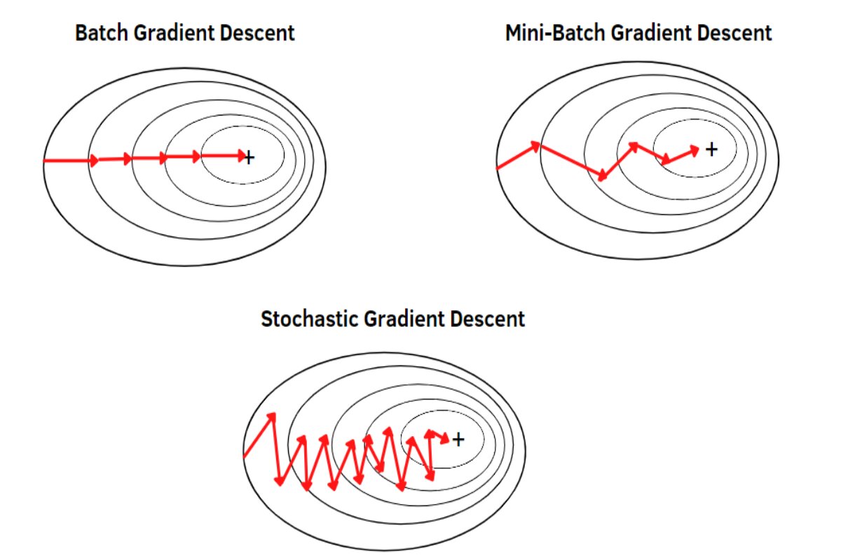
Mini-batch Gradient Descent is a compromise between Batch Gradient Descent (BGD) and Stochastic Gradient Descent (SGD). It involves updating the model’s parameters using a small subset (mini-batch) of the training dataset rather than the entire dataset or a single data point. This approach combines the advantages of both BGD and SGD.
Problem in Stochastic Gradient Descent (SGD):
High Variance Updates:
- In SGD, each parameter update is based on the gradient of a single randomly selected data point. This randomness can lead to updates with high variance, causing the optimization process to be noisy and fluctuate significantly.
- Because SGD relies on a single data point to calculate each update, the specific choice of that data point can greatly impact the direction and magnitude of the update. As a result, the optimization process becomes noisy, and the updates may fluctuate significantly from one iteration to the next.
Slow Convergence Near Optimum:
- In the final stages of optimization, when the model is close to the optimum, the high variance updates in SGD can lead to slow and erratic convergence. The noise introduced by single-data-point updates can make it difficult to zero in on the minimum.
Inefficient Hardware Utilization:
- Modern hardware, such as GPUs, benefits from parallel processing. However, SGD’s update-by-update nature might not efficiently utilize these resources.
- Modern hardware, particularly Graphics Processing Units (GPUs), is designed for parallel processing, which can significantly speed up computations. However, the traditional Stochastic Gradient Descent (SGD) optimization algorithm, with its update-by-update nature, may not fully exploit these hardware capabilities, leading to inefficient hardware utilization.
- The problem stems from the fact that SGD processes data points one at a time and updates model parameters sequentially. This sequential nature of updates can underutilize the parallel processing power of GPUs, which are capable of performing multiple calculations simultaneously. Consequently, GPUs may spend a considerable amount of time waiting for the next data point to arrive, leading to suboptimal hardware utilization and potentially slower training times.
How Mini-batch Gradient Descent Tackles These Problems:
Mini-batch Gradient Descent offers a solution that leverages the strengths of both SGD and Batch Gradient Descent (BGD)
Variance Reduction
Variance Reduction in Mini-batch Gradient Descent: In Mini-batch Gradient Descent, the training dataset is divided into smaller subsets known as mini-batches, each containing a fixed number of data points. When computing the gradient and updating model parameters, the algorithm considers the average gradient over the mini-batch. This averaging process inherently reduces the variance in parameter updates compared to the traditional Stochastic Gradient Descent (SGD) approach, which updates parameters using a single data point at a time. As a result, Mini-batch Gradient Descent tends to provide more stable and less erratic optimization, facilitating smoother convergence during the training of machine learning models.
Balanced Updates
- Balanced Updates in Mini-batch Gradient Descent: Mini-batch Gradient Descent strikes a balance between two extremes: the high variance updates of Stochastic Gradient Descent (SGD) and the stable updates of Batch Gradient Descent (BGD). This balance is achieved by dividing the training dataset into smaller subsets called mini-batches, each containing a fixed number of data points.
- By using these mini-batches, Mini-batch Gradient Descent provides more accurate gradient estimates compared to SGD, where a single data point is used for each update. This improved accuracy leads to more balanced and less erratic parameter updates during training. It combines the benefits of faster convergence from BGD and the noise-robustness of SGD, making it a widely adopted optimization technique for training machine learning models efficiently and effectively.
Faster Convergence:
- Faster Convergence with Mini-batch Gradient Descent: Mini-batch Gradient Descent updates the model’s parameters more frequently than Batch Gradient Descent (BGD), which can result in faster convergence during the training process. This is particularly noticeable in comparison to Stochastic Gradient Descent (SGD), where updates are based on single data points and can be noisy and erratic. Mini-batch Gradient Descent strikes a balance by considering small subsets of data (mini-batches) for parameter updates, combining the advantages of more frequent updates with reduced noise compared to SGD. As a result, it often achieves quicker convergence, making it a preferred choice for optimizing machine learning models efficiently.
Efficient Hardware Utilization:
- Efficient Hardware Utilization with Mini-batch Processing: Mini-batch processing in machine learning optimizes the utilization of modern hardware, such as GPUs, by enabling parallel computations on multiple data points within a mini-batch. This approach efficiently harnesses the parallel processing capabilities of the hardware, ensuring that multiple calculations can be performed simultaneously. As a result, it maximizes computational resource usage and accelerates training times, making it a practical choice for machine learning tasks on contemporary hardware architectures.
Choosing Mini-batch Size
- The choice of mini-batch size is crucial. Smaller batch sizes introduce more noise but can lead to faster convergence. Larger batch sizes reduce noise but might slow down convergence. Common choices are powers of 2 (e.g., 32, 64, 128) due to hardware optimization reasons.
- Mini-batch Gradient Descent addresses the problems of high variance updates, slow convergence near the optimum, and inefficient hardware utilization associated with Stochastic Gradient Descent. It offers a compromise between the stability of BGD and the speed of SGD, making it a widely used optimization algorithm in training deep learning models.
Here’s how Mini-batch Gradient Descent works in the context of deep learning
Initialization: Start by initializing the model’s parameters randomly.
Data Batching: Divide the training dataset into smaller subsets called mini-batches. Each mini-batch contains a fixed number of data points (e.g., 32, 64, 128) chosen randomly from the dataset.
Iteration: For each mini-batch, follow these steps:
Forward Pass
Perform a forward pass through the neural network for each data point in the mini-batch. Compute the model’s predictions using the current parameter values.
Calculate Average Loss
Calculate the average loss for the mini-batch. This is done by summing up the losses for each data point in the mini-batch and then dividing by the mini-batch size.
Calculate Gradients:
Calculate the gradients of the loss function concerning the model’s parameters based on the average loss of the mini-batch. These gradients indicate the direction and magnitude of change needed in the parameters to reduce the average loss.
Update Parameters: Update the model’s parameters based on the calculated gradients. The update is performed using the formula
new_parameter = old_parameter – learning_rate * gradient
Repeat: Repeat step 3 for each mini-batch in the training dataset. This completes one iteration (also known as an epoch).
Epochs: Repeat steps 2 to 4 for a predefined number of epochs or until the loss converges to a satisfactory level.
Benefits of Mini-batch Gradient Descent:
Faster Convergence
Similar to SGD, Mini-batch Gradient Descent offers faster convergence compared to BGD. It achieves this by taking advantage of larger mini-batches while maintaining more stable updates compared to pure SGD. Mini-batch Gradient Descent, as the name suggests, divides the training dataset into smaller subsets called mini-batches. Unlike BGD, which computes the gradient on the entire dataset before updating the model, Mini-batch Gradient Descent computes the gradient on a mini-batch and updates the model more frequently.
Mini-batch Gradient Descent takes advantage of parallelism in modern hardware, such as GPUs. It processes multiple data points simultaneously within each mini-batch. This parallelism accelerates the gradient computation and parameter updates, leading to faster convergence.
Regularized Updates
Mini-batch Gradient Descent combines elements of both BGD and SGD. While BGD provides stable updates by considering the entire dataset, it can be slow due to infrequent updates. On the other hand, pure SGD updates the model very frequently, but this can introduce a lot of noise. Mini-batch SGD strikes a balance by updating the model with the average gradient over a mini-batch. This provides more stability compared to pure SGD but faster convergence compared to BGD.
Improved Generalization
Mini-batch Gradient Descent often leads to better generalization than pure SGD because it utilizes more data in each update. This helps to average out noise in the loss landscape and find a more representative path to a good solution.
Smoothing of Trajectory:
The use of mini-batches results in a smoother trajectory of the optimization process. In contrast, pure SGD can exhibit highly erratic trajectories as it responds to the noise introduced by individual data points. This smoother trajectory makes it easier for the optimization to converge to a good solution. Mini-batch training is more robust in this regard because it averages over a mini-batch of points, reducing the influence.
Vectorized Operations
Deep learning frameworks and numerical libraries have optimized implementations of mathematical operations that are highly compatible with GPU hardware. These libraries can perform operations on entire mini-batches as opposed to individual data points. This vectorization allows for efficient GPU usage, resulting in faster training times
In deep learning frameworks like TensorFlow and PyTorch, mathematical operations are implemented as highly optimized, low-level operations on tensors (multi-dimensional arrays). These operations are executed efficiently making Mini-batch SGD well-suited for modern computational platforms.
Batched Operations
Mini-batch Gradient Descent is scalable, meaning it can handle datasets of various sizes. Whether you have a small or large dataset, you can adjust the mini-batch size accordingly to make efficient use of your hardware resources. Mini-batch processing allows for batch operations, which are more efficient than processing one data point at a time. GPUs can efficiently perform the same operation on multiple data points in parallel, significantly reducing the per-operation overhead. While GPUs provide massive parallelism, they also have limited memory. Mini-batch Gradient Descent aids in memory efficiency by loading and processing a smaller subset of the data at a time.
This means that you can train on datasets that may not fit entirely in GPU memory by carefully managing the mini-batch size. Mini-batch Gradient Descent reduces the noise inherent in SGD by processing a small, randomly selected subset of the data (the mini-batch) at a time. By averaging the gradients computed over the mini-batch, you get a more representative estimate of the true gradient of the loss function.
In Mini-batch SGD, the gradient computation and parameter updates are performed for each mini-batch, rather than for every individual data point. This reduces the overhead associated with updating model parameters, as it’s done less frequently compared to pure Stochastic Gradient Descent (SGD).
When using Mini-batch SGD, you load and preprocess a small batch of data at a time. This means you don’t need to load the entire dataset into memory, which can be crucial when dealing with large datasets that may not fit in RAM. Instead, you load and process data incrementally, reducing memory requirements.
Scaling with Hardware
As hardware advances and becomes more parallelized, the efficiency of Mini-batch Gradient Descent also improves. Newer GPUs with more cores and better parallel processing capabilities can further speed up training when using mini-batches. Mini-batch SGD is especially compatible with GPUs, which are highly parallel processors. Neural network training with Mini-batch SGD can be significantly accelerated when run on GPU hardware. GPUs are designed to perform many parallel computations simultaneously, and the mini-batch approach leverages this capability effectively. As mentioned, some hardware, particularly GPUs, may perform optimally with mini-batch sizes that are powers of 2 (e.g., 32, 64, 128). This is because GPUs are designed to process data in chunks that align with their architecture. Choosing such sizes can lead to better hardware utilization and faster training
The computational resources you have at your disposal also play a role. If you have access to powerful GPUs or TPUs, you can often use larger mini-batches because these accelerators can process them efficiently. Conversely, if you’re limited to CPUs, you might need to use smaller mini-batches to avoid excessive memory usage and slow computation.
Adaptability
Mini-batch sizes can be adjusted based on the available computational resources. Larger batch sizes are more efficient but might lead to slower convergence due to smaller updates. Smaller batch sizes can increase the update frequency but might be computationally expensive.
Choosing Mini-batch Size
The size of your dataset is a primary consideration. For small datasets, you can afford to use larger mini-batches, whereas for larger datasets, you might opt for smaller mini-batches due to memory constraints and computational efficiency. The choice of mini-batch size depends on factors like dataset size, model complexity, and available hardware. Smaller batch sizes introduce more noise but can lead to faster convergence, while larger batch sizes reduce noise but might slow down convergence. Common choices are powers of 2 (e.g., 32, 64, 128) due to hardware optimization reasons.
The complexity of your model can influence the choice of mini-batch size. Complex models with many parameters might require smaller mini-batches to converge efficiently. Simpler models may handle larger mini-batches.
Noise vs. Convergence Trade-off
Smaller mini-batches introduce more noise into the gradient estimates because they are computed over fewer data points. This noise can help the optimization process escape local minima but might slow down convergence due to erratic updates. On the other hand, larger mini-batches provide smoother gradient estimates, reducing the noise but potentially leading to slower convergence. In pure SGD, the model parameters are updated after processing each data point. This frequent updating can introduce a significant amount of noise into the learning process. Noise can cause the optimization process to oscillate or converge slowly because the updates can be in different directions for each data point.
Although Mini-batch Gradient Descent introduces some noise compared to BGD (which computes gradients on the entire dataset), this noise is typically less disruptive than the noise in pure SGD. The mini-batch size is chosen to be small enough to introduce some noise for exploration but large enough to smooth out some of the noise present in SGD. This balance aids in achieving a faster and more stable convergence. The use of mini-batches helps stabilize the learning process by reducing the noise introduced by SGD’s single-data-point updates.
.
Mini-batch Gradient Descent strikes a balance between Batch Gradient Descent and Stochastic Gradient Descent. It offers faster convergence and better computational efficiency, making it a widely used optimization algorithm for training deep learning models on large datasets.
Advantages and disadvantages of mini-batch gradient
Advantages
Efficient Parallel Processing
Mini-batch Gradient Descent divides the dataset into smaller mini-batches, allowing for parallel computation of gradients on modern hardware like GPUs. This speeds up training by processing multiple data points simultaneously.
Faster Convergence
Compared to Batch Gradient Descent, Mini-batch Gradient Descent updates parameters more frequently due to smaller batch sizes. This can lead to faster convergence and quicker adjustments to model weights.
Memory Efficiency
Mini-batches are smaller than the entire dataset, requiring less memory. This makes it possible to train on larger datasets that might not fit entirely in memory.
Generalization Improvement
The noise introduced by mini-batch updates helps models escape local minima and overfitting, leading to better generalization.
Disadvantages
Learning Rate Selection
Choosing an appropriate learning rate for Mini-batch Gradient Descent can still be challenging. A learning rate that’s too high can cause the optimization process to diverge, while one that’s too low can lead to slow convergence.
Batch Size Selection
Selecting the right mini-batch size is crucial. Small batch sizes introduce more noise but might converge faster, while larger batch sizes reduce noise but might slow down convergence.
Parameter Tuning
Mini-batch Gradient Descent introduces additional hyperparameters to tune, such as batch size and learning rate, which might require experimentation.
Complexity
Implementing Mini-batch Gradient Descent can be more complex than standard Gradient Descent due to the need to manage mini-batches and adaptively update learning rates.
Let’s solve one simple example
Data
(x₁, y₁) = (1, 3.5)
(x₂, y₂) = (2, 6.8)
(x₃, y₃) = (3, 9.9)
(x₄, y₄) = (4, 12.3)
(x₅, y₅) = (5, 15.5)
Initialize θ to 0
Learning Rate (α) = 0.01
Mini-batch Size (B) = 2
Iteration 1
Randomly select a mini-batch of size B = 2. Let’s say we select (x₁, y₁) and (x₂, y₂).
Compute the gradient for this mini-batch
Gradient for data point 1: ∇J(θ; x₁) = -(3.5 – θ * 1) * 1
Gradient for data point 2: ∇J(θ; x₂) = -(6.8 – θ * 2) * 2
Update θ using the average gradient information computed from the mini-batch
θ’ = θ – α * (1/2) * (∇J(θ; x₁) + ∇J(θ; x₂))
Now, calculate the new θ
θ’ = θ – 0.01 * (1/2) * [-3.5 + θ + (-13.6 + 2θ)]
θ’ = θ – 0.01 * (-8.55 + θ)
θ’ = θ + 0.0001 * (8.55 – θ)
Cost Function Update
Now, let’s calculate the cost function (J(θ)) at each iteration and observe how it decreases:
Cost Function at Iteration 1: J(θ) ≈ 68.7027
Parameter Update
θ at Iteration 1: θ’ ≈ 0.0001 * (8.55 – θ)
Iteration 2
Randomly select another mini-batch of size B = 2. Let’s say we select (x₃, y₃) and (x₄, y₄).
Compute the gradient for this mini-batch
Gradient for data point 3: ∇J(θ; x₃) = -(9.9 – θ * 3) * 3
Gradient for data point 4: ∇J(θ; x₄) = -(12.3 – θ * 4) * 4
Update θ using the average gradient information computed from the mini-batch
θ’ = θ – α * (1/2) * (∇J(θ; x₃) + ∇J(θ; x₄))
Now, calculate the new θ
θ’ = θ – 0.01 * (1/2) * [-29.7 + 3θ – 49.2 + 4θ]
θ’ = θ – 0.01 * (-78.9 + 7θ)
θ’ = θ + 0.0001 * (78.9 – 7θ)
Cost Function Update
Cost Function at Iteration 2: J(θ) ≈ 66.8593
Parameter Update
θ at Iteration 2: θ’ ≈ 0.0001 * (78.9 – 7θ)
Iteration 3
Randomly select another mini-batch of size B = 2. Let’s say we select (x₅, y₅) and (x₁, y₁).
Compute the gradient for this mini-batch
Gradient for data point 5: ∇J(θ; x₅) = -(15.5 – θ * 5) * 5
Gradient for data point 1: ∇J(θ; x₁) = -(3.5 – θ * 1) * 1
Update θ using the average gradient information computed from the mini-batch
θ’ = θ – α * (1/2) * (∇J(θ; x₅) + ∇J(θ; x₁))
Now, calculate the new θ
θ’ = θ – 0.01 * (1/2) * [-77.5 + 6θ + (-3.5 + θ)]
θ’ = θ – 0.01 * (-81 + 7θ)
θ’ = θ + 0.0001 * (81 – 7θ)
Cost Function Update
Cost Function at Iteration 3: J(θ) ≈ 61.7328
Parameter Update
θ at Iteration 3: θ’ ≈ 0.0001 * (81 – 7θ)
Iteration 4
Randomly select another mini-batch of size B = 2. Let’s say we select (x₂, y₂) and (x₄, y₄).
Compute the gradient for this mini-batch
Gradient for data point 2: ∇J(θ; x₂) = -(6.8 – θ * 2) * 2
Gradient for data point 4: ∇J(θ; x₄) = -(12.3 – θ * 4) * 4
Update θ using the average gradient information computed from the mini-batch
θ’ = θ – α * (1/2) * (∇J(θ; x₂) + ∇J(θ; x₄))
Now, calculate the new θ
θ’ = θ – 0.01 * (1/2) * [(-13.6 + 2θ) + (-49.2 + 4θ)]
θ’ = θ – 0.01 * (-61.6 + 6θ)
θ’ = θ + 0.0006 * (61.6 – 6θ)
Cost Function Update
Cost Function at Iteration 4: J(θ) ≈ 55.1182
Parameter Update
θ at Iteration 4: θ’ ≈ 0.0006 * (61.6 – 6θ)
Iteration 5
Randomly select another mini-batch of size B = 2. Let’s say we select (x₅, y₅) and (x₁, y₁).
Compute the gradient for this mini-batch
Gradient for data point 5: ∇J(θ; x₅) = -(15.5 – θ * 5) * 5
Gradient for data point 1: ∇J(θ; x₁) = -(3.5 – θ * 1) * 1
Update θ using the average gradient information computed from the mini-batch
θ’ = θ – α * (1/2) * (∇J(θ; x₅) + ∇J(θ; x₁))
Now, calculate the new θ
θ’ = θ – 0.01 * (1/2) * [-77.5 + 6θ + (-3.5 + θ)]
θ’ = θ – 0.01 * (-81 + 7θ)
θ’ = θ + 0.0001 * (81 – 7θ)
Cost Function Update
Cost Function at Iteration 5: J(θ) ≈ 52.5109
Parameter Update
θ at Iteration 5: θ’ ≈ 0.0001 * (81 – 7θ)
Now, you have the parameter values (θ) and cost function values at each iteration up to Iteration 5. The cost function is decreasing with each iteration, indicating that the model is converging toward a minimum. The specific values of θ and the cost function will continue to evolve as you perform more iterations, gradually reaching convergence.
Conclusion
Mini-batch Gradient Descent offers advantages like efficient parallel processing, faster convergence, memory efficiency, and generalization improvement. However, it also presents challenges such as learning rate and batch size selection, additional hyperparameter tuning, and increased complexity in implementation. Despite these limitations, Mini-batch Gradient Descent strikes a balance between the stability of Batch Gradient Descent and the speed of Stochastic Gradient Descent, making it a widely used optimization method for training deep learning models, especially in scenarios like image classification with CNNs.
Mini-batch Gradient Descent is a compromise between regular Gradient Descent and Stochastic Gradient Descent. Instead of using the entire dataset (as in regular Gradient Descent) or just one data point (as in Stochastic Gradient Descent), Mini-batch Gradient Descent computes gradients and updates the model parameters using small batches of data points. This approach combines some of the benefits of both methods, allowing for a balance between computation efficiency and convergence speed. Here’s the mathematical explanation of Mini-batch Gradient Descent:


