OptiLearn: Mastering Gradient Descent
Gradient Descent is a fundamental optimization algorithm widely used in training deep learning models. It’s a process that helps the model find the optimal set of parameters (weights and biases) to minimize the loss function, which measures the difference between predicted and actual values.
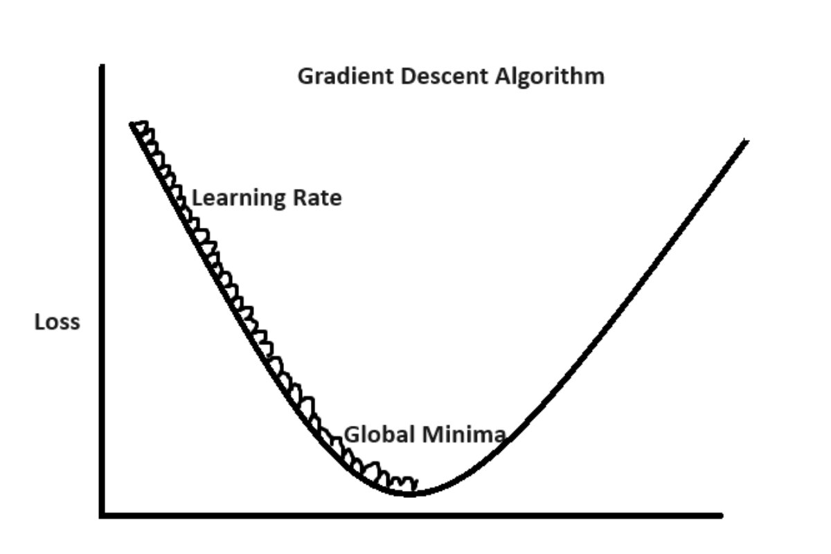
Gradient Descent is used to minimize a function, typically a loss function, by iteratively adjusting the parameters of a model. The algorithm computes the gradient of the function concerning the model parameters and updates the parameters in the direction that leads to a decrease in the function’s value.
Gradient Descent is a foundational optimization technique, and it forms the basis for many advanced optimization algorithms used in deep learning, such as Stochastic Gradient Descent (SGD), Mini-batch SGD, and Adam. These variations introduce techniques to enhance convergence speed, handle noisy gradients, and adapt learning rates dynamically.
Steps to use gradient descent algorithm.
Initialization:
Start by initializing the model’s parameters randomly. These parameters determine how the model transforms input data into predictions.
Forward Pass:
For each training data point, perform a forward pass through the neural network. This involves applying the model’s transformations to the input data, layer by layer, to generate predictions.
Calculate Loss:
Compare the model’s predictions with the actual target values from the training dataset. Use an appropriate loss function (e.g., Mean Squared Error for regression or Cross-Entropy for classification) to quantify the difference between predictions and targets.
Calculate Gradients:
Compute the gradients of the loss function concerning each model parameter. Gradients represent the direction and magnitude of change needed in each parameter to decrease the loss. This involves backpropagation, where you calculate the gradient of the loss concerning each layer’s output, and then recursively calculate gradients for the previous layers.
Update Parameters:
Adjust the model’s parameters based on the calculated gradients. This adjustment is performed to reduce the loss in the next iteration. The formula for updating each parameter is:
new_parameter = old_parameter – learning_rate * gradient
Here, the learning rate is a hyperparameter that determines the step size of each parameter update. It’s a crucial factor in determining the convergence speed and stability of the optimization process.
Repeat:
Repeat steps 2 to 5 for a predefined number of iterations (epochs) or until the loss converges to a satisfactory level.
Convergence:
As you iterate through the training process, the loss should decrease over time. The model’s parameters are adjusted in a way that aligns predictions more closely with target values.
Validation:
Periodically evaluate the model’s performance on a validation dataset to ensure that it’s not overfitting. If the performance of the validation data starts degrading, consider techniques like early stopping or regularization.
Test:
After training is complete, evaluate the model’s performance on a separate test dataset to assess its generalization ability on unseen data.
Let’s understand it with a simple example.
Step 1: Initialization
Initialize the model parameters θ₀ and θ₁ to arbitrary values. Let’s start with:
θ₀ = 0.5
θ₁ = 1.0
Step 2: Compute Gradient
Calculate the gradient of the Mean Squared Error (MSE) loss function concerning θ₀ and θ₁. The formula for MSE is:
MSE = (1/n) * Σ(yᵢ – ŷᵢ)²
Where:
- n is the number of data points
- yᵢ is the actual target value for the i-th data point
- ŷᵢ is the predicted value for the i-th data point
- For a linear regression model, ŷᵢ is given by:
- ŷᵢ = θ₀ + θ₁ * xᵢ
We also need to compute the gradients:
∂MSE/∂θ₀ = (-2/n) * Σ(yᵢ – ŷᵢ)
∂MSE/∂θ₁ = (-2/n) * Σ(yᵢ – ŷᵢ) * xᵢ
For simplicity, let’s assume we have the following data points:
Data Point 1: (x₁ = 1.0, y₁ = 2.0)
Data Point 2: (x₂ = 2.0, y₂ = 3.0)
Using our initial parameter values, we calculate ŷᵢ for each data point:
ŷ₁ = 0.5 + 1.0 * 1.0 = 1.5
ŷ₂ = 0.5 + 1.0 * 2.0 = 2.5
Now, we can calculate the gradient for θ₀ and θ₁:
∂MSE/∂θ₀ = (-2/2) * [(2.0 – 1.5) + (3.0 – 2.5)] = -0.5
∂MSE/∂θ₁ = (-2/2) * [(2.0 – 1.5) * 1.0 + (3.0 – 2.5) * 2.0] = -1.5
Step 3: Update Parameters
Update the model parameters θ₀ and θ₁ using the learning rate α. Let’s assume α = 0.1 for this example.
θ₀’ = θ₀ – α * ∂MSE/∂θ₀ = 0.5 – 0.1 * (-0.5) = 0.55
θ₁’ = θ₁ – α * ∂MSE/∂θ₁ = 1.0 – 0.1 * (-1.5) = 1.15
Step 4: Repeat
Repeat steps 2 and 3 iteratively until convergence. We’ll perform one more iteration:
Calculate ŷᵢ using the updated parameters:
ŷ₁ = 0.55 + 1.15 * 1.0 = 1.7
ŷ₂ = 0.55 + 1.15 * 2.0 = 2.85
Calculate the new gradients:
∂MSE/∂θ₀ = (-2/2) * [(2.0 – 1.7) + (3.0 – 2.85)] ≈ -0.225
∂MSE/∂θ₁ = (-2/2) * [(2.0 – 1.7) * 1.0 + (3.0 – 2.85) * 2.0] ≈ -0.325
Update the parameters:
θ₀’ = 0.55 – 0.1 * (-0.225) ≈ 0.5725
θ₁’ = 1.15 – 0.1 * (-0.325) ≈ 1.1825
Step 5: Repeat (Iteration 4)
Calculate ŷᵢ using the updated parameters:
ŷ₁ = 0.5725 + 1.1825 * 1.0 ≈ 1.755
ŷ₂ = 0.5725 + 1.1825 * 2.0 ≈ 2.9405
Calculate the new gradients:
∂MSE/∂θ₀ ≈ -0.175
∂MSE/∂θ₁ ≈ -0.2725
Update the parameters:
θ₀’ ≈ 0.5725 – 0.1 * (-0.175) ≈ 0.590725
θ₁’ ≈ 1.1825 – 0.1 * (-0.2725) ≈ 1.209775
Step 6: Repeat (Iteration 5)
Calculate ŷᵢ using the updated parameters:
ŷ₁ ≈ 1.755 + 1.209775 * 1.0 ≈ 1.964775
ŷ₂ ≈ 1.755 + 1.209775 * 2.0 ≈ 3.17455
Calculate the new gradients:
∂MSE/∂θ₀ ≈ -0.080225
∂MSE/∂θ₁ ≈ -0.158325
Update the parameters:
θ₀’ ≈ 0.590725 – 0.1 * (-0.080225) ≈ 0.598748
θ₁’ ≈ 1.209775 – 0.1 * (-0.158325) ≈ 1.225581
Step 7: Repeat (Iteration 6)
Calculate ŷᵢ using the updated parameters:
ŷ₁ ≈ 1.964775 + 1.225581 * 1.0 ≈ 2.190356
ŷ₂ ≈ 1.964775 + 1.225581 * 2.0 ≈ 3.415937
Calculate the new gradients:
∂MSE/∂θ₀ ≈ -0.046633
∂MSE/∂θ₁ ≈ -0.091162
Update the parameters:
θ₀’ ≈ 0.598748 – 0.1 * (-0.046633) ≈ 0.603411
θ₁’ ≈ 1.225581 – 0.1 * (-0.091162) ≈ 1.234697
Step 8: Repeat (Iteration 7)
Calculate ŷᵢ using the updated parameters:
ŷ₁ ≈ 2.190356 + 1.234697 * 1.0 ≈ 2.425053
ŷ₂ ≈ 2.190356 + 1.234697 * 2.0 ≈ 3.660750
Calculate the new gradients:
∂MSE/∂θ₀ ≈ -0.030045
∂MSE/∂θ₁ ≈ -0.058907
Update the parameters:
θ₀’ ≈ 0.603411 – 0.1 * (-0.030045) ≈ 0.606416
θ₁’ ≈ 1.234697 – 0.1 * (-0.058907) ≈ 1.240587
Step 9: Repeat (Iteration 8)
Calculate ŷᵢ using the updated parameters:
ŷ₁ ≈ 2.425053 + 1.240587 * 1.0 ≈ 2.665640
ŷ₂ ≈ 2.425053 + 1.240587 * 2.0 ≈ 3.906227
Calculate the new gradients:
∂MSE/∂θ₀ ≈ -0.020638
∂MSE/∂θ₁ ≈ -0.040414
Update the parameters:
θ₀’ ≈ 0.606416 – 0.1 * (-0.020638) ≈ 0.608480
θ₁’ ≈ 1.240587 – 0.1 * (-0.040414) ≈ 1.244628
Step 10: Repeat (Iteration 9)
Calculate ŷᵢ using the updated parameters:
ŷ₁ ≈ 2.665640 + 1.244628 * 1.0 ≈ 2.910268
ŷ₂ ≈ 2.665640 + 1.244628 * 2.0 ≈ 4.154895
Calculate the new gradients:
∂MSE/∂θ₀ ≈ -0.014557
∂MSE/∂θ₁ ≈ -0.028531
Update the parameters:
θ₀’ ≈ 0.608480 – 0.1 * (-0.014557) ≈ 0.609935
θ₁’ ≈ 1.244628 – 0.1 * (-0.028531) ≈ 1.245481
Step 11: Repeat (Iteration 10)
Calculate ŷᵢ using the updated parameters:
ŷ₁ ≈ 2.910268 + 1.245481 * 1.0 ≈ 3.155749
ŷ₂ ≈ 2.910268 + 1.245481 * 2.0 ≈ 4.401229
Calculate the new gradients:
∂MSE/∂θ₀ ≈ -0.010074
∂MSE/∂θ₁ ≈ -0.019733
Update the parameters:
θ₀’ ≈ 0.609935 – 0.1 * (-0.010074) ≈ 0.610943
θ₁’ ≈ 1.245481 – 0.1 * (-0.019733) ≈ 1.246454
We continue the process in the same manner. Over time, the updates become smaller, and the parameters θ₀ and θ₁ approach their optimal values. The number of iterations required for convergence depends on factors like the learning rate and the specific problem. After many iterations, the loss function will converge to a minimum value, and the parameters θ₀ and θ₁ will stabilize. These optimal parameter values represent the best-fitting linear model for the given data, minimizing the Mean Squared Error (MSE).
Advantages and disadvantages of Gradient Descent.
Advantages:
Convergence to Local Minima:
- Gradient Descent aims to minimize the loss function iteratively. It usually converges to a local minimum of the loss function, effectively finding the best-fitting parameters for the model.
Applicability to Large Datasets:
- Gradient Descent processes data in batches, making it suitable for large datasets. Mini-batch or stochastic variants can further speed up training by utilizing parallel processing.
Flexibility:
- Gradient Descent can be applied to various models, including neural networks and other machine learning algorithms.
Continuous Improvement:
- With each iteration, the algorithm fine-tunes the model’s parameters, leading to gradual improvement in the model’s fit to the data.
Disadvantages/Limitations:
Choice of Learning Rate:
- Selecting an appropriate learning rate is crucial. A learning rate that’s too small can lead to slow convergence, while one that’s too large can cause the optimization process to overshoot the minimum or even diverge.
Local Minima and Saddle Points:
- Gradient Descent can get stuck in local minima or saddle points, where the gradient is close to zero but the algorithm hasn’t yet reached the global minimum.
Sensitivity to Initialization:
- The starting point of the optimization can impact the final solution. Different initializations might lead to different local minima.
- Slow Convergence on Poorly Conditioned Problems: Gradient Descent can converge slowly on loss surfaces with narrow, elongated valleys, especially if the learning rate isn’t carefully chosen.
Noise and Stochasticity:
- Stochastic Gradient Descent can introduce noise due to random sampling of data points. This noise can cause oscillations or slower convergence.
Conclusion:
Gradient Descent has numerous advantages, including its ability to converge to local minima, applicability to large datasets, and continuous improvement. However, it also comes with limitations such as the sensitivity to learning rate, potential convergence to local minima, and noise introduced by stochasticity. These limitations often lead to the development of more advanced optimization algorithms, like Mini-batch Gradient Descent, Momentum, and Adam, which attempt to address some of the challenges associated with traditional Gradient Descent methods.


