StatusNeo

Distribution in Data Science

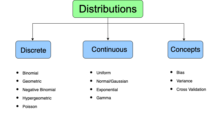
Discrete

1. Binomial

x successes in n events, each with p probability

with μ = np and σ² = npq

	=	binomial probability
	=	number of times for a selected outcome within n trials
	=	number of combinations
	=	probability of success on one trial
	=	probability of failure on a one-trial
	=	number of trials

Note: If n = 1, this can be a Bernoulli distribution

---

2. Geometric

Geometric distribution may be a variety of opportunity distribution supported three key assumptions. These are arranged as follows.

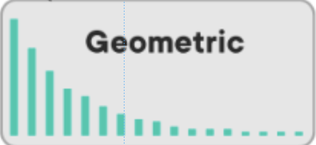
• The tests performed are independent.
• There are often only two results for every trial – success or failure.
• The probability of success, indicated by p, is that the same for every test.

 first success with p probability on the n^th trial

qⁿ⁻¹p, with µ = 1/p and σ² =^1−p/p²

---

3. Negative Binomial

• A negative binomial distribution (also called the Pascal Distribution) for random variables in a negative binomial experiment.

• number of failures before r successes

---

4. Hypergeometric

• The hypergeometric distribution is very the same as the statistical distribution. In fact, Bernoulli distribution is a superb measure of hypergeometric distribution as long as you create a sample of fifty or less of the population.

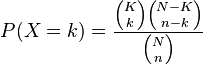
• K is that the number of successes within the population
• k is that the number of observed successes
• N is that the population size
• n is that the number of draws
• X is items of that feature

---

5. Poisson

number of successes x in a hard and fast quantity, where success occurs at a median rate

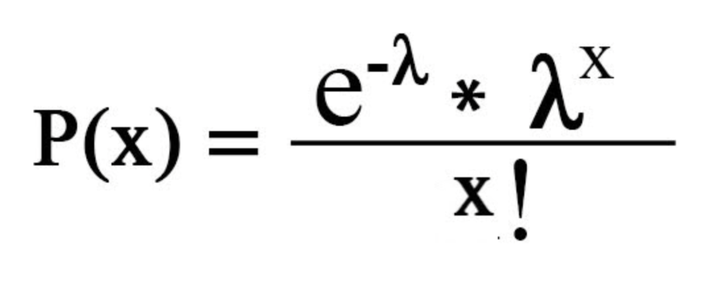
 µ = σ² = λ

---

---

Continuous

1. Uniform

all values between a and b are equally likely

f(x)=1/(b−a)

for a ≤ x ≤ b

Theoretical definition formulas and standard deviations are present

μ=(a+b)/2 and σ=√(b−a)²/12

---

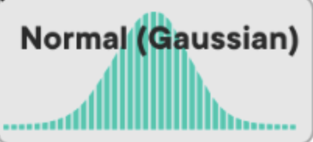
2. Normal/Gaussian

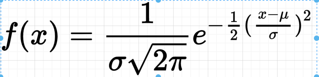
	=	Probability density function
	=	Standard deviation
	=	Mean

Central Limit Theorem – sample mean of i.i.d. data approaches Gaussian distribution.

Empirical Rule – 68%, 95%, and 99.7% of values lie within one, two, and three standard deviations of the mean.

Normal Approximation – discrete distributions like Binomial and Poisson may be approximated using z-scores when np, nq, and λ are greater than 10

---

3. Exponential

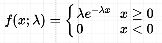
	=	probability density function
	=	rate parameter
	=	Random variable

memoryless time between independent events occurring at a median rate λ → λe^−λx, with µ = 1/λ

---

4. Gamma

time until n independent events occurring at a mean rate λ

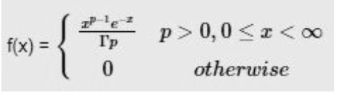
where p and x are continuous chance variable.

Γ(α) = Gamma function

---

---

Concepts

Prediction Error = Bias² + Variance + Irreducible Noise

1. Bias

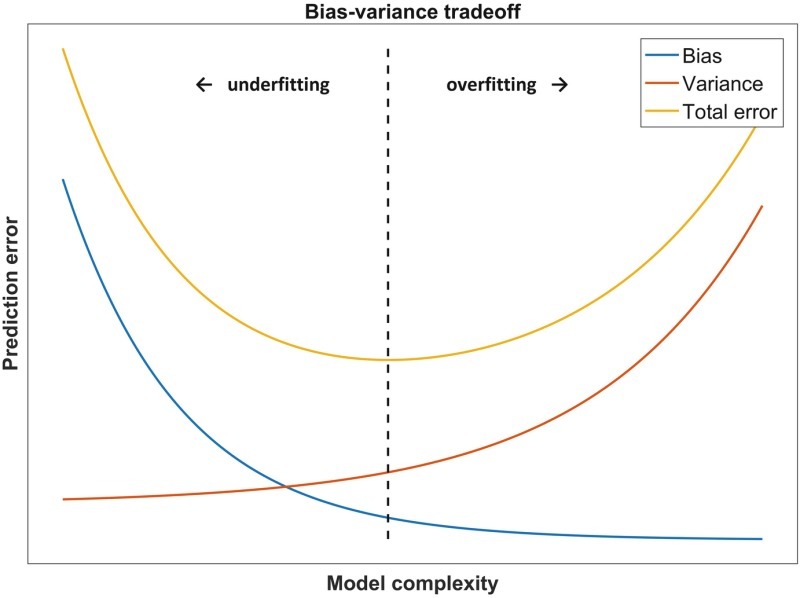
wrong assumptions when training → can’t capture underlying patterns → underfit

2. Variance

sensitive to fluctuations when training→ can’t generalize on unseen data → overfit 

The bias-variance tradeoff attempts to attenuate these two sources of error, through methods such as: 

– Cross-validation to generalize to unseen data

– Dimension reduction and have selection 

In all cases, as variance decreases, bias increases.

ML models may be divided into two types: 

– Parametric – uses a hard and fast number of parameters with regard to sample size 

– Non-Parametric – uses a versatile number of parameters and doesn’t make particular assumptions on the data

3. Cross-Validation

validates test error with a subset of coaching data, and selects parameters to maximize average performance-

– k-fold – divide data into k groups, and use one to validate

– leave-pout – use p samples to validate and also the rest to train

Reference:- https://github.com/aaronwangy/Data-Science-Cheatsheet