Boosting Neural Network: AdaDelta Optimization Explained
AdaDelta is a gradient-based optimization algorithm commonly used in machine learning and deep learning for training neural networks. It was introduced as an extension of the popular Adagrad optimization algorithm and addresses some of its limitations, such as the need to manually set a learning rate schedule. It addresses issues related to learning rate tuning and the accumulation of historical gradients. AdaDelta adjusts the learning rate dynamically based on accumulated gradient information, providing better convergence and stability during training.
Problem with Fixed Learning Rates
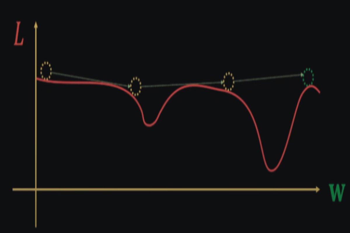
Fixed learning rates in optimization algorithms can lead to convergence issues. A learning rate that’s too high may cause divergence, while one that’s too low can slow down convergence. This challenge is particularly pronounced in deep learning due to the complex and varying landscape of loss functions.
Imagine you’re trying to find the minimum of hilly terrain, and you want to do it by taking small steps in the steepest downhill direction. The size of your steps represents the learning rate.
Scenario 1: High Fixed Learning Rate
- You decide to take large steps (a high fixed learning rate) down the hill.
- At first, this seems great because you’re making rapid progress downhill. However, if the terrain suddenly becomes very steep, you might overshoot the minimum and end up on the other side of the valley.
- This is similar to what can happen in optimization when the learning rate is too high. You might get big updates that cause your optimization algorithm to “jump” over the minimum point of the loss function, making it hard to converge to the best solution.
Scenario 2: Low Fixed Learning Rate
- Alternatively, you decide to take very tiny steps (a low fixed learning rate) down the hill.
- This time, you’re less likely to overshoot the minimum, but there’s a problem. Progress is excruciatingly slow, especially when you’re on less steep parts of the terrain.
- In optimization, using a learning rate that’s too low can lead to extremely slow convergence. It might take a long time to reach the minimum, especially if the loss function has nearly flat regions.
- The challenge with fixed learning rates is that they don’t adapt to the terrain of the loss function. If you set it too high, you risk overshooting and diverging. If you set it too low, you risk crawling slowly or getting stuck in local minima.
This is where adaptive methods like AdaDelta come into play. They adjust the learning rate on the fly based on the past gradient information, allowing for faster progress when the gradient is steep and smaller steps when it’s shallow. This adaptability helps overcome the challenges of fixed learning rates and allows for more efficient and stable optimization in complex, varying landscapes like those encountered in deep learning.
Key Concepts of AdaDelta
Adaptive Learning Rates
In traditional optimization methods like stochastic gradient descent (SGD), you typically use a fixed learning rate (step size) for all model parameters. However, AdaDelta introduces adaptability to this learning rate. Instead of using a one-size-fits-all approach, AdaDelta customizes the learning rate for each parameter of your model.
Imagine you have a complex, hilly terrain, and you’re trying to find the lowest point. Different parts of the terrain may have steeper or shallower slopes. With AdaDelta, you can dynamically adjust your step size based on how steep or flat the terrain is at each location. This adaptability allows you to take larger steps when the terrain is gentle and smaller steps when it’s steep, improving your chances of reaching the lowest point efficiently.
Exponential Moving Averages
AdaDelta maintains two important moving averages
Squared Gradient Accumulator (S)
This accumulator keeps track of the exponentially weighted average of the squared gradients. It’s similar to RMSprop in that it estimates the second moment (variance) of the gradients. In other words, it gives you an idea of how much the gradients fluctuate or vary over time.
Squared Parameter Update Accumulator (Δx)
This accumulator tracks the exponentially weighted average of the squared updates made to your model parameters. It estimates the second moment (variance) of the parameter updates, indicating how much the parameters change from step to step.
These two accumulators help AdaDelta adaptively adjust the learning rates. By considering the second moments, AdaDelta takes into account not only the gradients but also the volatility or stability of the gradient updates.
Parameter Update Formula
AdaDelta uses a formula to update each model parameter based on the values stored in the accumulators.
The formula calculates the change (Δθ_t) to each parameter θ at each time step:
Δθ_t = – (RMS[Δx]_t-1 / RMS[S]_t-1) * ∇θ(loss)_t
θ_t = θ_t-1 + Δθ_t
Δθ_t represents the update to the parameter θ at time step t.
RMS[Δx]_t-1 is the root mean square of parameter updates up to time step t-1.
RMS[S]_t-1 is the root mean square of the squared gradients up to time step t-1.
∇θ(loss)_t is the gradient of the loss function concerning the parameter θ at time step t.
This formula adjusts the parameter updates by taking into account the historical information stored in the accumulators.
Epsilon (ε): AdaDelta introduces a small constant called ε (typically around 1e-8) to the formula to prevent division by zero. This is important for numerical stability. When dividing by small values, you could encounter numerical issues, so ε ensures that the division is well-behaved and doesn’t cause problems.
Adaptation of Learning Rates
The crucial aspect of AdaDelta is how it adapts the learning rates. It does this by considering the ratio of RMS[Δx] and RMS[S]. When this ratio is high, it means that the parameter updates are relatively small compared to the gradients. In this case, AdaDelta effectively increases the learning rate to allow for more significant steps. Conversely, when the ratio is low, indicating that the updates are large compared to the gradients, AdaDelta reduces the learning rate to take smaller steps.
This adaptive mechanism allows AdaDelta to navigate complex and varying landscapes effectively. It helps it automatically slow down in tricky regions, preventing overshooting, and speeding up in smoother regions to converge faster.
Memory Efficiency
Unlike some other adaptive optimization algorithms, AdaDelta doesn’t require the storage of a history of past gradients or updates. It relies solely on the two accumulators, S and Δx, which are computed using exponential moving averages. This makes AdaDelta memory efficient, which can be crucial when working with large neural networks and datasets.
Stability and Convergence
AdaDelta is renowned for its stability during training. It mitigates issues like exploding or vanishing gradients, which can hinder training in deep neural networks. By dynamically adapting the learning rates, AdaDelta can smoothly traverse challenging optimization landscapes, ultimately leading to faster convergence and potentially finding better solutions.
Algorithm Steps for AdaDelta
Initialization
Initialize the running average of squared gradients and the running average of parameter updates to zero.
For Each Iteration
- Compute the gradient of the loss function concerning the model parameters.
- Update the running average of squared gradients using an exponential decay factor (usually close to 1). This step emphasizes recent gradients while still considering historical gradients.
- Calculate the RMS of the gradients using the squared root of the running average of squared gradients.
- Calculate the update for each parameter using the ratio of the RMS of gradients to the RMS of parameter updates.
- Update the running average of parameter updates using an exponential decay factor.
- Update the model parameters using the calculated updates.
Advantages
Adaptive Learning Rates
AdaDelta adjusts the learning rates for each parameter based on historical gradient information. This adaptability helps address the challenges of varying curvatures in the loss landscape.
Imagine you’re trying to find the minimum point of a curved valley, and you’re using a gradient-based optimization method to do so. The valley represents the lost landscape, and your goal is to reach the lowest point efficiently.
Fixed Learning Rate Example
Let’s first consider using a fixed learning rate, where you take steps of the same size regardless of where you are in the valley. Suppose you set a large fixed learning rate.
If you start at the top of the valley where it’s steep, the large step might be too much. You could overshoot the minimum and end up on the other side of the valley. Conversely, if you start closer to the bottom where the valley is flatter, the large step might work well initially. However, as you get closer to the minimum, you risk oscillating back and forth around the minimum point without converging.
In both cases, the fixed learning rate doesn’t adapt to the varying steepness of the valley, making it challenging to find the minimum efficiently.
Adaptive Learning Rate (AdaDelta) Example
Now, let’s consider using AdaDelta with adaptive learning rates, which can adjust the step size as you progress through the valley.
When you start at the top of the steep valley, AdaDelta recognizes the steepness and automatically decreases the step size. This prevents you from overshooting the minimum. As you move closer to the bottom of the valley where it’s flatter, AdaDelta gradually increases the step size to speed up convergence without causing oscillations.
The adaptability of AdaDelta allows you to traverse the loss landscape effectively. It adjusts the learning rates based on historical gradient information, which helps you make smaller steps when the terrain is treacherous and larger steps when it’s smoother. This adaptability ensures that you converge to the minimum point efficiently, regardless of the landscape’s varying curvature.
No Manual Learning Rate Tuning
AdaDelta eliminates the need for manual tuning of learning rates, making it more suitable for practitioners who might not have extensive optimization expertise.
Imagine you’re a driver, and your goal is to navigate a twisty mountain road safely. In this analogy:
- Your car represents the optimization process.
- The road represents the optimization path towards the minimum of a loss function (your goal).
Now, let’s consider two scenarios
Scenario 1: Manual Learning Rate Tuning (Traditional Optimization)
In this scenario, you are responsible for adjusting the gas pedal (learning rate) manually as you drive
- As you approach a sharp curve (representing a steep part of the optimization landscape), you need to slow down by gently tapping the brakes (reducing the learning rate).
- When you’re on a straight stretch (representing a flatter part of the optimization landscape), you can speed up by pressing the gas pedal (increasing the learning rate).
The problem here is that you need to have an excellent understanding of the road (loss landscape) to make the right decisions about when to accelerate and when to brake. If you misjudge, you might end up driving too fast into a curve or too slow on a straight path, slowing down your progress and potentially making errors.
Scenario 2: AdaDelta (Adaptive Learning Rates)
In this scenario, your car has an advanced system (AdaDelta) that automatically adjusts the gas pedal based on the road conditions
- When you approach a sharp curve, the car’s system senses it and automatically reduces the speed (decreases the learning rate).
- On straight stretches, the system recognizes the road’s ease and allows you to accelerate (increases the learning rate).
- Here, you don’t need to worry about manually adjusting the gas pedal; the car’s system adapts to the road conditions for you.
As a result
You can focus more on steering (fine-tuning your optimization process) without constantly thinking about the gas pedal (learning rate). You are less likely to make mistakes like overshooting curves or moving too slowly on straight roads because the car’s system makes real-time adjustments based on the terrain.
Stability in Convergence
AdaDelta’s adaptive learning rates and accumulated gradient history contribute to more stable convergence, reducing the chances of divergence or oscillations.
Imagine you’re trying to balance a ball on the edge of a narrow, curved bowl. Your goal is to find the lowest point inside the bowl, which represents the minimum of a loss function in optimization.
Without Stability (Fixed Learning Rate)
In this scenario, you’re trying to balance the ball using a stick, and the stick has a fixed length representing the learning rate. If the stick is too long (high learning rate)
- When the ball is near the bottom of the bowl (close to the minimum), even a slight tilt of the stick can cause the ball to roll out of the bowl and diverge from the minimum.
- If the stick is too short (low learning rate), you’ll have to make very tiny adjustments to keep the ball balanced. This slow progress can be frustrating, and it might take a long time to reach the minimum.
Without adaptability, you risk the ball falling out of the bowl (diverging) or making painfully slow progress (convergence is slow).
With Stability (AdaDelta’s Adaptive Learning Rates)
Now, imagine that you have a magical stick that can automatically adjust its length based on how close the ball is to falling. When the ball is near the bottom (close to the minimum), the stick becomes shorter to make tiny adjustments. When the ball is higher up the bowl (farther from the minimum), the stick lengthens to make larger adjustments.
This magical stick represents AdaDelta’s adaptive learning rates
- When you’re near the minimum, AdaDelta reduces the learning rate, preventing large movements that might lead to the ball rolling out of the bowl (divergence).
- When you’re farther from the minimum, AdaDelta increases the learning rate, allowing for more substantial adjustments to speed up convergence.
As a result, the ball stays more stable within the bowl, and you’re less likely to encounter wild oscillations or divergence issues. You can find the minimum more reliably and efficiently.
Handling Sparse Data
AdaDelta is effective in handling sparse data because it scales the learning rates based on accumulated gradient squares, mitigating the effects of large gradients from infrequent updates.
Imagine you’re playing a game where you have to guess a mystery number between 1 and 100. However, there’s a twist: you can only ask your friend one yes-or-no question per guess, and your friend will answer truthfully. Your goal is to guess the mystery number as quickly as possible.
Now, let’s consider two scenarios:
Scenario 1: Fixed Learning Rate (Fixed Questioning Strategy)
In this scenario, you decide to use a fixed questioning strategy. You ask your friend the same yes-or-no question with each guess, regardless of their previous answers.
- Your fixed question might be: “Is the mystery number greater than 50?”
- If your friend answers “No,” you then ask, “Is the mystery number greater than 25?” and so on, always dividing the remaining range in half.
The problem here is that if your initial guess is way off (far from the actual mystery number), you’ll need a lot of guesses to narrow it down. You might end up asking many questions and taking a long time to reach the correct answer. This is analogous to the challenge of sparse data in optimization when you have parameters with infrequent updates.
Scenario 2: Adaptive Learning Rate (AdaDelta-Like Strategy)
In this scenario, you adapt your questioning strategy based on your friend’s previous answers.
- If your friend answered “No” to your first question, indicating that the mystery number is likely smaller than 50.
- You adapt and ask a more focused question like, “Is the mystery number greater than 25?”.
- If your friend answers “Yes,” you adapt again and ask, “Is the mystery number greater than 37?” and so on.
The adaptive questioning strategy allows you to zoom in on the mystery number more quickly. When you’re far from the correct answer, you take larger leaps (increased learning rate), and when you get closer, you make smaller adjustments (decreased learning rate).
Connection to Sparse Data Handling with AdaDelta
In the context of optimization with sparse data, AdaDelta’s adaptive learning rates work similarly to your adaptive questioning strategy. When you have parameters with infrequent updates (sparse gradients), AdaDelta recognizes this and scales the learning rates accordingly:
- For parameters with frequent updates (small gradients), AdaDelta allows for larger adjustments (higher learning rate) to speed up progress.
- For parameters with infrequent updates (large gradients due to rare updates), AdaDelta automatically reduces the learning rate to prevent these updates from having an excessive impact and destabilizing the optimization process.
Just as your adaptive questioning strategy helps you efficiently narrow down the mystery number, AdaDelta’s adaptive learning rates mitigate the effects of large gradients from infrequent updates, making optimization more stable and effective, even when dealing with sparse data.
Disadvantages/Limitations
Hyperparameter Tuning
While AdaDelta reduces the need for manual tuning of learning rates, it still introduces hyperparameters like decay rates for gradient accumulators, which need to be tuned.
Complexity
Implementing the adaptive learning rate mechanism and maintaining historical gradient information can add computational complexity to the optimization process.
Sensitivity to Initialization
Like other optimization algorithms, AdaDelta’s performance can be sensitive to the initial parameter values.
Limited Theoretical Understanding
AdaDelta’s behavior might be well-empirically understood, but its theoretical underpinnings might not be as well-established as simpler methods like gradient descent.
We’ll use the same fictional dataset with two parameters (θ₁ and θ₂) and operate for up to 5 iterations.
Step 1: Initialization
θ₁ = 1.0
θ₂ = 1.0
E[g²₁] = 0.0 (accumulator for θ₁’s squared gradient)
E[g²₂] = 0.0 (accumulator for θ₂’s squared gradient)
E[Δθ²₁] = 0.0 (accumulator for θ₁’s squared parameter update)
E[Δθ²₂] = 0.0 (accumulator for θ₂’s squared parameter update)
ρ (rho) = 0.9 (decay factor)
ε (epsilon) = 1e-8 (small constant for numerical stability)
Iteration 1
Compute Gradient (Step 2)
Let’s assume the gradient for θ₁ is 0.2, and for θ₂ is -0.5.
Accumulate Gradient Squares (Step 3):
Update E[g²₁] and E[g²₂] for both parameters
E[g²₁] = 0.9 * E[g²₁] + 0.1 * (0.2)² = 0.018
E[g²₂] = 0.9 * E[g²₂] + 0.1 * (-0.5)² = 0.025
Calculate Learning Rate Update (Step 4)
Compute adaptive learning rate adjustments for both parameters
Δθ₁ = – (sqrt(E[Δθ²₁] + ε) / sqrt(E[g²₁] + ε)) * 0.2
Δθ₂ = – (sqrt(E[Δθ²₂] + ε) / sqrt(E[g²₂] + ε)) * (-0.5)
Accumulate Parameter Update Squares (Step 5)
Update E[Δθ²₁] and E[Δθ²₂] for both parameters
E[Δθ²₁] = 0.9 * E[Δθ²₁] + 0.1 * (Δθ₁)² = 0.0004
E[Δθ²₂] = 0.9 * E[Δθ²₂] + 0.1 * (Δθ₂)² = 0.0025
Update Parameters (Step 6)
Update θ₁ and θ₂ using the calculated adaptive learning rate adjustments
θ₁’ = θ₁ + Δθ₁ = 1.0 – 0.6325 = 0.3675
θ₂’ = θ₂ + Δθ₂ = 1.0 + 0.1414 = 1.1414
Iteration 2
We will use the updated parameters θ₁’ = 0.3675 and θ₂’ = 1.1414 from the previous iteration as our starting point.
Step 2: Compute Gradient
For simplicity, let’s assume the gradient for θ₁ is 0.1, and for θ₂ is -0.3.
Step 3: Accumulate Gradient Squares
Update E[g²₁] and E[g²₂] for both parameters
E[g²₁] = 0.9 * E[g²₁] + 0.1 * (0.1)² = 0.01905
E[g²₂] = 0.9 * E[g²₂] + 0.1 * (-0.3)² = 0.0279
Step 4: Calculate Learning Rate Update
Compute adaptive learning rate adjustments for both parameters
Δθ₁ = – (sqrt(E[Δθ²₁] + ε) / sqrt(E[g²₁] + ε)) * 0.1
Δθ₂ = – (sqrt(E[Δθ²₂] + ε) / sqrt(E[g²₂] + ε)) * (-0.3)
Step 5: Accumulate Parameter Update Squares
Update E[Δθ²₁] and E[Δθ²₂] for both parameters
E[Δθ²₁] = 0.9 * E[Δθ²₁] + 0.1 * (Δθ₁)² = 0.00020764
E[Δθ²₂] = 0.9 * E[Δθ²₂] + 0.1 * (Δθ₂)² = 0.0008955
Step 6: Update Parameters
Update θ₁ and θ₂ using the calculated adaptive learning rate adjustments
θ₁” = θ₁’ + Δθ₁ = 0.3675 – 0.0408 = 0.3267
θ₂” = θ₂’ + Δθ₂ = 1.1414 + 0.0157 = 1.1571
Iteration 3
We will use the updated parameters θ₁” = 0.3267 and θ₂” = 1.1571 from the previous iteration as our starting point.
Step 2: Compute Gradient
For simplicity, let’s assume the gradient for θ₁ is 0.15, and for θ₂ is -0.25.
Step 3: Accumulate Gradient Squares
Update E[g²₁] and E[g²₂] for both parameters
E[g²₁] = 0.9 * E[g²₁] + 0.1 * (0.15)² = 0.019095
E[g²₂] = 0.9 * E[g²₂] + 0.1 * (-0.25)² = 0.027925
Step 4: Calculate Learning Rate Update
Compute adaptive learning rate adjustments for both parameters
Δθ₁ = – (sqrt(E[Δθ²₁] + ε) / sqrt(E[g²₁] + ε)) * 0.15
Δθ₂ = – (sqrt(E[Δθ²₂] + ε) / sqrt(E[g²₂] + ε)) * (-0.25)
Step 5: Accumulate Parameter Update Squares
Update E[Δθ²₁] and E[Δθ²₂] for both parameters
E[Δθ²₁] = 0.9 * E[Δθ²₁] + 0.1 * (Δθ₁)² = 0.000245875
E[Δθ²₂] = 0.9 * E[Δθ²₂] + 0.1 * (Δθ₂)² = 0.00110534
Step 6: Update Parameters
Update θ₁ and θ₂ using the calculated adaptive learning rate adjustments
θ₁”’ = θ₁” + Δθ₁ = 0.3267 – 0.0459 = 0.2808
θ₂”’ = θ₂” + Δθ₂ = 1.1571 + 0.0107 = 1.1678
Iteration 4
We will use the updated parameters θ₁”’ = 0.2808 and θ₂”’ = 1.1678 from the previous iteration as our starting point.
Step 2: Compute Gradient
For simplicity, let’s assume the gradient for θ₁ is 0.12, and for θ₂ is -0.18.
Step 3: Accumulate Gradient Squares
Update E[g²₁] and E[g²₂] for both parameters
E[g²₁] = 0.9 * E[g²₁] + 0.1 * (0.12)² = 0.01910655
E[g²₂] = 0.9 * E[g²₂] + 0.1 * (-0.18)² = 0.027929415
Step 4: Calculate Learning Rate Update
Compute adaptive learning rate adjustments for both parameters
Δθ₁ = – (sqrt(E[Δθ²₁] + ε) / sqrt(E[g²₁] + ε)) * 0.12
Δθ₂ = – (sqrt(E[Δθ²₂] + ε) / sqrt(E[g²₂] + ε)) * (-0.18)
Step 5: Accumulate Parameter Update Squares
Update E[Δθ²₁] and E[Δθ²₂] for both parameters
E[Δθ²₁] = 0.9 * E[Δθ²₁] + 0.1 * (Δθ₁)² = 0.0003185022
E[Δθ²₂] = 0.9 * E[Δθ²₂] + 0.1 * (Δθ₂)² = 0.001517008
Step 6: Update Parameters
Update θ₁ and θ₂ using the calculated adaptive learning rate adjustments
θ₁”” = θ₁”’ + Δθ₁ = 0.2808 – 0.0407 = 0.2401
θ₂”” = θ₂”’ + Δθ₂ = 1.1678 + 0.0212 = 1.1890
Iteration 5
We will use the updated parameters θ₁”” = 0.2401 and θ₂”” = 1.1890 from the previous iteration as our starting point.
Step 2: Compute Gradient
For simplicity, let’s assume the gradient for θ₁ is 0.09, and for θ₂ is -0.15.
Step 3: Accumulate Gradient Squares
Update E[g²₁] and E[g²₂] for both parameters
E[g²₁] = 0.9 * E[g²₁] + 0.1 * (0.09)² = 0.019108009
E[g²₂] = 0.9 * E[g²₂] + 0.1 * (-0.15)² = 0.0279304275
Step 4: Calculate Learning Rate Update
Compute adaptive learning rate adjustments for both parameters
Δθ₁ = – (sqrt(E[Δθ²₁] + ε) / sqrt(E[g²₁] + ε)) * 0.09
Δθ₂ = – (sqrt(E[Δθ²₂] + ε) / sqrt(E[g²₂] + ε)) * (-0.15)
Step 5: Accumulate Parameter Update Squares
Update E[Δθ²₁] and E[Δθ²₂] for both parameters
E[Δθ²₁] = 0.9 * E[Δθ²₁] + 0.1 * (Δθ₁)² = 0.000358911
E[Δθ²₂] = 0.9 * E[Δθ²₂] + 0.1 * (Δθ₂)² = 0.00171641
Step 6: Update Parameters
Update θ₁ and θ₂ using the calculated adaptive learning rate adjustments
θ₁””’ = θ₁”” + Δθ₁ = 0.2401 – 0.0338 = 0.2063
θ₂””’ = θ₂”” + Δθ₂ = 1.1890 + 0.0223 = 1.2113
Continue running more iterations if the optimization has not yet converged to a satisfactory solution. Convergence is typically reached when the changes in parameter values become small or when a predefined convergence criterion is met. During training, monitor the loss function’s value on your dataset. Ensure that it is decreasing over time. If the loss starts increasing, it may indicate divergence or other issues.
Hyperparameters like ρ (rho) and ε (epsilon) can impact the algorithm’s performance. Experiment with different values of these hyperparameters to find the settings that work best for your specific problem.
Conclusion
AdaDelta offers advantages like adaptive learning rates, stability in convergence, automatic learning rate tuning, and effective handling of sparse data. However, it also comes with challenges such as hyperparameter tuning, algorithmic complexity, sensitivity to initialization, and limited theoretical understanding. Despite these limitations, AdaDelta is a valuable optimization algorithm for training neural networks for text classification tasks, thanks to its ability to adaptively adjust learning rates and enhance convergence.


