Adaptive Gradient Optimization Explained
AdaGrad stands for Adaptive Gradient Algorithm. It is a popular optimization algorithm used in machine learning and deep learning for training models, especially in the context of gradient-based optimization methods for minimizing loss functions during training. AdaGrad was designed to automatically adapt the learning rates for individual parameters.
Adagrad (Adaptive Gradient Algorithm) aims to dynamically adjust the learning rates for each parameter based on the historical gradient information. Adagrad is particularly useful when dealing with sparse data and features with varying importance, as it adapts the learning rates individually for each parameter.
- Sparse data refers to data in which a large portion of the values are zero or missing. In a sparse dataset, most of the data points or features have no significant information or are empty, making them sparse in terms of non-zero or non-missing values. Sparse data is common in various fields, including natural language processing, recommendation systems, genomics, and more.
- In a sparse dataset, a significant portion of the values are zero or null, meaning they don’t contain meaningful information. Sparse data often leads to high-dimensional feature spaces because each unique non-zero value or category is treated as a distinct feature. This can pose challenges for machine learning algorithms that assume dense data.
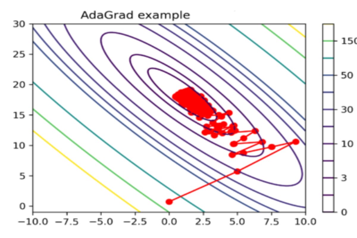
This adaptiveness helps in converging quickly on steep dimensions while progressing more cautiously on shallow ones. Due to the accumulation of squared gradients, the learning rate for each parameter in AdaGrad typically decreases over time, which can be beneficial for convergence in many cases.
Let’s delve deeper into how Adagrad works
Accumulated Gradient Squares
- Accumulated Gradient Squares, as employed by the Adagrad optimization algorithm, involve keeping a running sum of the squared gradient values for each parameter during the training of a machine learning model. This accumulation of squared gradients is a key component of Adagrad and serves the purpose of adapting the learning rates for individual parameters. Adagrad maintains a separate running total of the squared gradient values associated with each parameter. This means that for every parameter in the model, there is a cumulative sum of the squares of its past gradients.
- The accumulated gradient squares play a crucial role in determining the learning rate for each parameter. In the update step of Adagrad, the learning rate for a parameter is inversely proportional to the square root of the accumulated gradient squares for that parameter. In essence, parameters that have received larger gradients in the past will have their learning rates scaled down, while those with smaller gradients will have their learning rates scaled up.
Individual Learning Rates
- Unlike traditional optimization algorithms with a single learning rate for all parameters, Adagrad adapts the learning rate for each parameter individually based on the accumulated gradient information. Adagrad recognizes that not all model parameters should be updated at the same rate. It adapts the learning rate for each parameter according to its historical gradient behavior.
- Adagrad maintains a record of the squared gradients for each parameter over time. This information reflects how much each parameter has been changing in previous iterations. Parameters that have received larger gradient values in the past will have their learning rates reduced, while those with smaller gradients will have their learning rates increased.
- The use of individual learning rates allows Adagrad to converge effectively and efficiently, especially in scenarios with varying feature scales or sparse data. It ensures that the learning rates are tailored to the behavior of each parameter, preventing overly aggressive updates that may hinder convergence or overshoot the optimal solution.
Learning Rate Scaling
- Adagrad, to adjust the learning rate for individual model parameters during the training process. This technique involves scaling down the learning rate based on the historical behavior of the gradients. The learning rate for a particular parameter is scaled down by the square root of the sum of squared gradients for that parameter. Parameters that have large gradients will have smaller effective learning rates, while those with small gradients will have larger effective learning rates.
- Learning rate scaling is an adaptive mechanism that helps to prevent overshooting or convergence issues. Conversely, parameters with more stable or smaller gradients are allowed larger updates to facilitate convergence.
- Learning rate scaling is particularly useful in scenarios where the gradients across different parameters or features vary widely in magnitude. It allows the optimization algorithm to adapt to the specific behavior of each parameter, leading to more efficient convergence and better model performance.
Algorithm Steps for Adagrad
Initialization
Initialize the running sum of squared gradients for each parameter to a small positive value to avoid division by zero.
For Each Iteration
- Compute the gradient of the loss function concerning the model parameters.
- Update the running sum of squared gradients by adding the square of the current gradient for each parameter.
- Calculate the effective learning rate for each parameter by dividing the original learning rate by the square root of the running sum of squared gradients for that parameter.
- Update the parameters using the calculated gradient and the effective learning rate.
Benefits of Adagrad
Adaptive Learning Rates:
Adagrad adapts the learning rates individually for each parameter based on the historical gradient information. This allows it to automatically assign larger learning rates to parameters with smaller gradients and vice versa.
Faster convergence
- Parameters with smaller gradients can update more quickly, leading to faster convergence.
Stability
- Smaller learning rates for parameters with large gradients prevent overshooting and promote stability during optimization.
Customization
- The algorithm automatically tailors the learning rates to the specific characteristics of each parameter, making it suitable for problems with varying feature scales or sparse data.
Feature Importance Handling
In deep learning, some features might have more important gradients than others. Adagrad’s learning rates cater to this variation.
In many real-world datasets, some features have a more substantial impact on the model’s performance than others. These important features may have gradients that vary significantly from iteration to iteration, reflecting their influence on the optimization process. Conversely, less important features may have smaller, more stable gradients. By assigning customized learning rates to each feature, Adagrad ensures that the optimization process pays more attention to important features. Features with smaller gradients receive larger learning rates, allowing the model to update them more quickly, which can lead to faster convergence and better overall performance.
Sparse Data
Adagrad handles sparse data effectively because the learning rates are scaled based on the accumulated gradient squares, mitigating the issues of large gradients dominating updates. Traditional optimization algorithms often struggle with sparse data because they use a fixed learning rate for all parameters. In sparse datasets, a few non-zero gradients may result in very large updates for the corresponding parameters, potentially causing convergence issues or overshooting optimal solutions.
No Manual Learning Rate Tuning
No Manual Learning Rate Tuning” is a significant advantage of the Adagrad optimization algorithm. Adagrad automates the process of setting the learning rates for each parameter individually based on the accumulated gradient information, eliminating the need for manual intervention and tuning of learning rate hyperparameters.
Manual Learning Rate Tuning
- In traditional optimization algorithms, setting an appropriate learning rate (often denoted as η) is a critical but challenging aspect of training machine learning models. The learning rate determines the step size taken in the parameter space during each optimization iteration. If it’s too large, it can lead to overshooting and divergence, while if it’s too small, it can result in slow convergence or getting stuck in local minima.
Hyperparameter Tuning Challenges
- Finding the right learning rate can be a cumbersome and time-consuming process. Data scientists and machine learning practitioners often need to experiment with various learning rates through trial and error. This process involves multiple iterations of training and evaluating the model, making it computationally expensive and requiring domain expertise.
Adaptive Learning Rates in Adagrad
- Adagrad offers a solution to this problem by automatically adapting the learning rates for each parameter during training. It does this based on the historical gradient information for each parameter, as measured by the accumulation of squared gradients.
Benefits of Automatic Learning Rates
Simplicity
- Adagrad simplifies the training process by removing the need for manual learning rate tuning.
Efficiency
- It can converge more efficiently, even in situations where the optimal learning rate might change during training.
Generalization
- Automatic learning rate adaptation can lead to models that generalize better to unseen data, as they are less sensitive to the choice of a fixed learning rate.
Let’s see how it happens mathematically.
Step 1: Initialization
Initialize the model parameter θ to some initial value, and initialize an accumulator G to zero for each parameter, where G stores the sum of squared historical gradients. Also, set the learning rate α and ε for numerical stability.
Initial parameter: θ = 4
Initial accumulator: G = 0
Learning rate: α = 0.1
Epsilon: ε = 1e-8
Step 2: Compute Gradient
Calculate the gradient (g) of the loss function concerning the model parameter (θ). In this example, we use a simple quadratic loss function:
Loss function: L(θ) = (θ – 3)²
Gradient: g = dL(θ)/dθ = 2(θ – 3)
For the initial θ value (θ = 4), the gradient is:
g₁ = 2(4 – 3) = 2
Step 3: Accumulate Gradient Squares
Update the accumulator G for the parameter θ using the squared gradient:
G₁ = G + g₁² = 0 + 2² = 4
Step 4: Calculate Learning Rate Adjustment
Calculate the adaptive learning rate adjustment for θ:
θ’₁ = θ – (α / sqrt(G₁ + ε)) * g₁
θ’₁ = 4 – (0.1 / sqrt(4 + 1e-8)) * 2 ≈ 3.9995
Iteration 2
Step 2: Compute Gradient
For θ = 3.9995, calculate the gradient (g₂):
g₂ = 2(3.9995 – 3) ≈ 1.999
Step 3: Accumulate Gradient Squares
Update the accumulator G for θ:
G₂ = G₁ + g₂² ≈ 4 + 1.999² ≈ 7.996
Step 4: Calculate Learning Rate Adjustment
Calculate the adaptive learning rate adjustment for θ:
θ’₂ = θ – (α / sqrt(G₂ + ε)) * g₂
θ’₂ ≈ 3.9995 – (0.1 / sqrt(7.996 + 1e-8)) * 1.999 ≈ 3.9990
Iteration 3
Step 2: Compute Gradient
For θ = 3.9990, calculate the gradient (g₃):
g₃ = 2(3.9990 – 3) ≈ 1.998
Step 3: Accumulate Gradient Squares
Update the accumulator G for θ:
G₃ = G₂ + g₃² ≈ 7.996 + 1.998² ≈ 11.988
Step 4: Calculate Learning Rate Adjustment
Calculate the adaptive learning rate adjustment for θ:
θ’₃ ≈ 3.9990 – (0.1 / sqrt(11.988 + 1e-8)) * 1.998 ≈ 3.9985
Iteration 4
Step 2: Compute Gradient
For θ = 3.9985, calculate the gradient (g₄):
g₄ = 2(3.9985 – 3) ≈ 1.997
Step 3: Accumulate Gradient Squares
Update the accumulator G for θ:
G₄ = G₃ + g₄² ≈ 11.988 + 1.997² ≈ 15.979
Step 4: Calculate Learning Rate Adjustment
Calculate the adaptive learning rate adjustment for θ:
θ’₄ ≈ 3.9985 – (0.1 / sqrt(15.979 + 1e-8)) * 1.997 ≈ 3.9979
Iteration 5
Repeat the process for the fifth iteration:
Step 2: Compute Gradient
For θ = 3.9979, calculate the gradient (g₅):
g₅ = 2(3.9979 – 3) ≈ 1.996
Step 3: Accumulate Gradient Squares
Update the accumulator G for θ:
G₅ = G₄ + g₅² ≈ 15.979 + 1.996² ≈ 19.971
Step 4: Calculate Learning Rate Adjustment
Calculate the adaptive learning rate adjustment for θ:
θ’₅ ≈ 3.9979 – (0.1 / sqrt(19.971 + 1e-8)) * 1.996 ≈ 3.9974
These are the results of the first five iterations of Adagrad. The learning rate and parameter value are updated in each iteration based on the gradient and accumulated gradient squares. This adaptiveness allows Adagrad to efficiently converge towards the minimum of the loss function.
Adagrad accumulates squared gradients over time, which can lead to diminishing learning rates for frequently updated parameters. This can make the optimization process very slow. To address this, variations like RMSprop and Adam were developed, which use exponentially decaying averages of squared gradients to mitigate the excessive decrease in learning rates.
Conclusion:
The Adagrad algorithm adjusts the learning rates for each parameter individually based on the historical gradient magnitudes. This is beneficial for sparse data scenarios where some features might have infrequent updates. However, Adagrad can lead to decreasing learning rates over time, potentially causing slower convergence in later stages of training. This issue has motivated the development of other algorithms like RMSprop and Adam, which address this learning rate decay problem.


