Navigating Outliers for Accurate Data Analysis & Decisions

Navigating Outliers for Accurate Data Analysis & Decisions

In this blog, we are going to see info about the outliers in machine learning.

Definition of outliers
Types of Outliers
Understanding the impact of outliers
Finding outliers
Dealing with these outliers
Others

Suppose we have data of a company which contains data of its employees. Now look at the table below, After the salary of the first 5 employees, the salary of one employee is very high, it may be possible that the person who is the highest in wages is the company CEO, then obviously the same salary will be higher than all the others.

ID	Wages(in lakh)
1211	10
1089	13
1403	17
1704	14
10087	100

But in terms of data analysis, these are called outliers, because this number is very different from the rest of the numbers and is also very large.

We have two types of outliers: lower-end outliers and one is higher-end outliers. So now in the above example we have seen the highest number is called the higher-end outlier and if there was the lowest number in the same table then that number would have been known as the lower-end outlier. An outlier in a dataset is a value that significantly differs from the majority of other values.

Definition of Outlier:

Mathematically, an outlier can be defined as a data point that falls outside a certain range from the central tendency of the data, such as the mean or median.

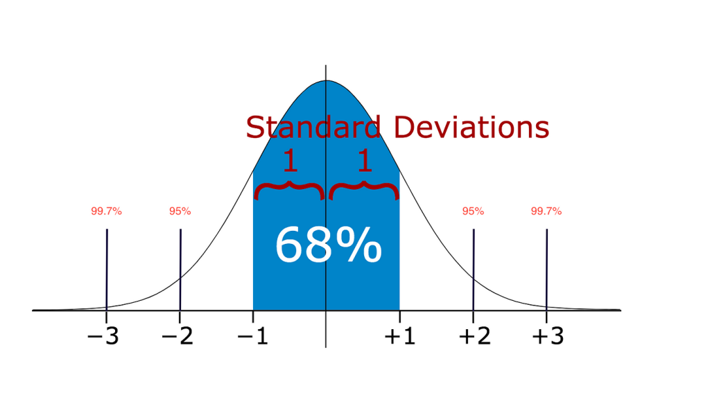
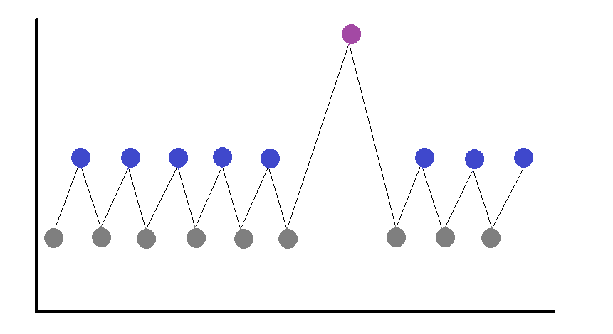
In the above figure, we can see a mean line, this is the mean point of the data set, and we can assume the data points are genuine up to the 3^rd standard deviation. Besides that, we assume the rest data points as outliers.

Outliers can indicate unusual or exceptional observations that might require further investigation to determine if they result from errors, anomalies, or genuinely unique occurrences within the data.

We have 3 types of outliers:

1. Global
2. collective
3. Contextual

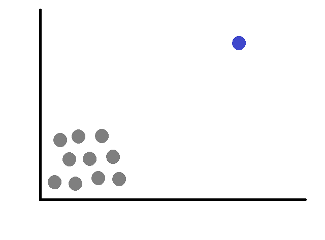
1. Global

In this, we find data in which all the numbers are close to each other or maybe within a particular limit and there is only one number that is far away from the rest, these are called global outliers.

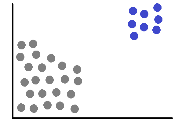
2. Collective:

In this, we find the same data as above and everything is the same as above, the only difference is that the long outlier is not alone, but it is also a group. It means collective.

3. Contextual:

In this, we come across data in which we see everything well, but at one point there is a big dip or rise in the data, and this is sudden rather than always.

To understand this, let’s look at an example, let’s say we have the data of a TV channel company called Star Gold on how many people watch this channel while looking at the data we get, we see the average data for 11 months of the year, but there is a single month that is the highest. It is because the IPL series was there in that month, so it can be seen that the channel got a lot of increase in customer base at that time. In another example, while the share market is going up continuously, the market falls suddenly and very deep.

But it’s important to note that with these types of outliers, we have some others too.

Data Entry Error >> Human Errors:

Imagine a teacher recording the scores of students on a recent test. The scores are as follows: 85, 92, 88, 78, 96, 89, 105, 91, 84, 90.
In this example, the score of 105 is a potential outlier that might have been caused by a data entry error. It’s important to investigate such outliers to ensure the data’s accuracy and reliability, especially when they could be due to human errors.

Measurement Errors >> Machine Error / Instrument Errors:

Imagine in a laboratory measuring the weight of apples using a digital scale. The true weights of the apples are 150g, 152g, 148g, 155g, 147g, 154g, 500g, 151g, 149g, and 153g.
In this example, the measurement of 500 is a potential outlier that might have been caused by a machine or instrument error. It’s crucial to investigate such outliers to ensure the accuracy and reliability of the measurement process, especially when they could result from errors in the measuring equipment.

Intentional Errors >> Dummy Dataset:

Imagine a teacher conducting an experiment in a science class, measuring the heights of students (in centimeters) as part of a lesson on data analysis. The actual heights are: 150 cm, 152 cm, 148 cm, 155 cm, 147 cm, 154 cm, 151 cm, 149 cm, 153 cm, and 156 cm.
However, for this example, the teacher decides to introduce an intentional error to test students’ ability to identify outliers.
So as decided to add an intentionally wrong measurement, she added 180 cm to the dataset to see if students could identify this outlier.
So now the new dataset becomes: 150 cm, 152 cm, 148 cm, 155 cm, 147 cm, 154 cm, 151 cm, 149 cm, 153 cm, 156 cm, and 180 cm.

Sampling Errors >> Mixing data from the wrong resources:

Imagine a researcher studying the average income of people in a small town. He decided to collect data from two different sources: a local job fair and a high-end business conference, interested in understanding the average income of the town’s residents, but these two sources represent very different groups within the town.
From the local job fair, he gathers income data for 100 people. Their incomes range from $25,000 to $60,000. And from the high-end business conference, he gathers income data for 50 people. Their incomes range from $80,000 to $300,000.
While analyzing the dataset, he noticed some extremely high values, such as $300. These values are outliers that don’t fit the overall pattern of the data.

These outliers were introduced due to the mixing of data from the high-end business conference. The extreme incomes from the conference group heavily influenced the mean, pulling it upwards. However, these outliers don’t accurately represent the town’s average income because they come from a different group within the town.

The mixing of data from the wrong resources led to sampling errors in analysis. These errors caused outliers to appear in the dataset and skewed the results. If he had only used the data from the local job fair, the average income of the town’s residents would have been much lower. On the other hand, if he had only used the data from the high-end business conference, the average income would have been much higher.

To avoid such errors, it’s important to carefully select data sources and ensure they represent the population we want to study. Mixing data from different groups can lead to misleading results and incorrect conclusions. Always consider the context and characteristics of the data sources before combining them

Natural Errors >> Most of the actual data belongs to the Natural Errors:

Imagine a wildlife researcher studying the heights of a population of deer in a forest, he collected data on their heights and was interested in understanding the typical height of these deer. However, natural variations can introduce errors in the data due to factors such as age, genetics, and environmental conditions.
he measured the heights of 50 deer in the forest. Heights range from 120 cm to 160 cm.
Some of the shorter deer might be fawns, while the taller ones might be mature adults.
As he analyzes the data, he might notice some deer that are significantly taller or shorter than the others. These extreme values are outliers that can arise due to natural variations in the population.
So, I want to emphasize that when you do this, you don’t jump to any conclusions without fully studying what you’re working on, consulting with your colleagues, why is this data point here, what is the reason for it is here, or why. It’s an outlier.

Understanding the impact of outliers:

To understand how outliers impact on model, let’s look below:

In the below example, we took one feature as age and target as salary. Here in the first example, we took all values closest to each other, which means here we are not using any outliers.

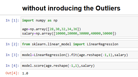
The accuracy of the above model is =1.0

Now in the second example, let’s add only one outlier, and let’s check how the model behaves.

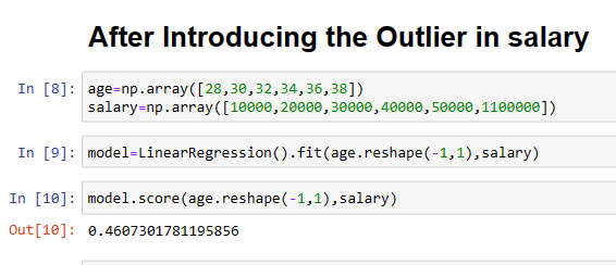
Because of the outlier, our accuracy is decreased and the final accuracy that we gain is = 0.46

Outliers affects:

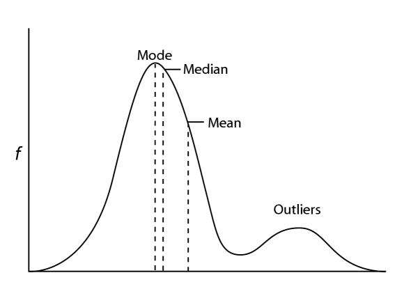
Mean (Average):

The mean is the sum of all data points divided by the total count. Outliers, especially if they’re much larger or smaller than the majority, can distort the mean. When an extreme value is present, it can “pull” the mean towards it, giving a false impression of the data’s central tendency. For instance, if most people earn around (10, 13, 14, 17) but a CEO’s salary of 100 is included, the mean income becomes much higher than what most people earn.

Median:

The median is the middle value in a sorted dataset. Outliers have less impact on the median because it’s not sensitive to extreme values. If there are a few very high or low values, they won’t drastically affect the middle value. This makes the median a better measure of the “typical” value in datasets with outliers.

Outliers can distort relationships and trends between variables:

1. Strength of Relationship:

An outlier with an extreme value in both variables can exaggerate the strength of their relationship. For instance, in a study about height and shoe size, an extremely tall person might make the relationship between the two variables appear stronger than it is.

2. Direction of Relationship:

Similarly, an outlier can make a relationship appear more positive or negative than it is. If most data points show a weak positive trend, one high outlier can make the relationship seem stronger.

3. Regression Models:

In linear regression, outliers can significantly impact the slope and fit of the regression line. If a single data point is far from the others, it can disproportionately influence the line’s position, potentially leading to a misleading interpretation of the relationship between variables.

4. Misleading Conclusions:

Representativeness: Outliers, by their nature, don’t represent the majority of the data. Relying on conclusions drawn from data with outliers can be misleading, as these extreme values might not reflect the typical behavior or pattern in the majority of cases.

Outlier Effect on Models:

Normal Distribution Assumption:

Many statistical tests assume that data follows a normal distribution (bell curve). Outliers can violate this assumption, leading to incorrect results and potentially causing significant differences to appear less significant or vice versa.

Model Performance:

Outliers can influence the performance of statistical models like linear regression. These models try to minimize the differences between predicted and actual values. An outlier with a large actual value might make the model focus too much on it, leading to poor predictions for other, more typical data points.

Overfitting:

Outliers can lead to overfitting in machine learning models. Overfitting occurs when a model becomes too complex and fits the training data too closely, capturing noise and extreme values. This makes the model less likely to generalize well to new, unseen data.

Bias:

Outliers can introduce bias into machine learning algorithms. For instance, algorithms like k-means clustering that rely on distances can be affected by outliers, leading to inaccurate cluster assignments.

Finding outliers:

We can find the outliers in various ways, like using the graphical way and using some mathematical way.

Let’s see some graphical way:

Scatter Plot:

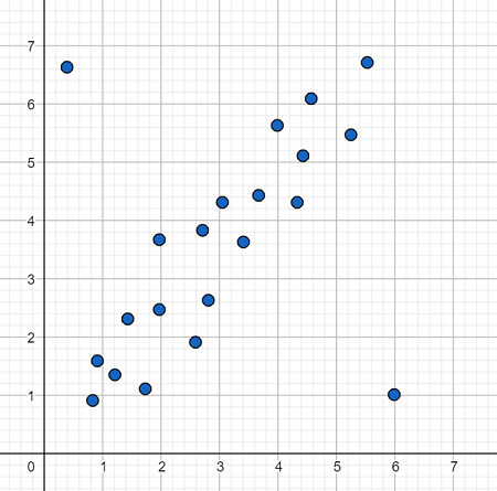
Scatter plots are especially useful when dealing with two variables. They display data points as individual dots on a graph, with one variable on the x-axis and another on the y-axis.
Outliers in a scatter plot can be identified as data points that deviate significantly from the general pattern formed by the rest of the data.
If most points cluster closely together, but one or a few points are situated far away from the main cluster, those distant points might be outliers.

Bar Plot:

1. Taller Bars:

If you see a bar that is much taller than the neighboring bars, it suggests that there might be an unusually high number of data points in that interval. These could potentially be outliers.

2. Shorter Bars:

Conversely, if you see a bar that is much shorter than the neighboring bars, it suggests that there might be very few data points in that interval. These intervals could also contain outliers.

3. Multiple Outliers:

If you notice multiple tall or short bars, this might indicate the presence of several outliers in different intervals.

Box Plot:

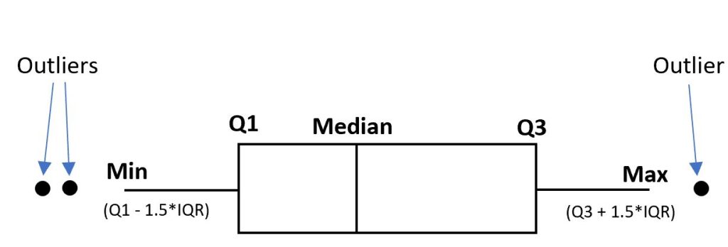
A box plot is a powerful visualization tool that gives you insights into the distribution of your data and helps you spot outliers. It consists of a rectangular box (the interquartile range or IQR) and “whiskers” that extend to the minimum and maximum values within a certain range.
The central line within the box represents the median, which is the middle value when the data is sorted.
The box itself spans the interquartile range (IQR), which covers the middle 50% of the data.
“Whiskers” extend from the box to show the range within which most of the data falls. Points outside this range are often considered potential outliers.
Individual points beyond the whiskers are plotted individually. These are points that might be outliers based on their distance from the rest of the data.

Q-Q Plot:

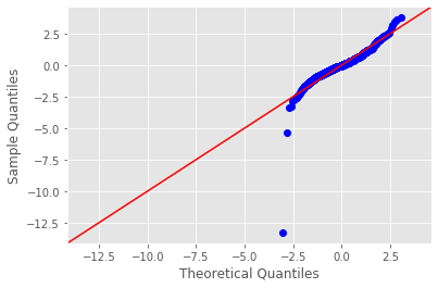
Q-Q plots are used to assess whether your data follows a particular theoretical distribution, often a normal distribution. They compare the quantiles of your data to the quantiles of the theoretical distribution.
If the points on a Q-Q plot form a roughly straight line, it indicates that your data follows the theoretical distribution.
Outliers in a Q-Q plot can be identified if they deviate significantly from the expected straight line at the tails of the distribution.

Violin Plot:

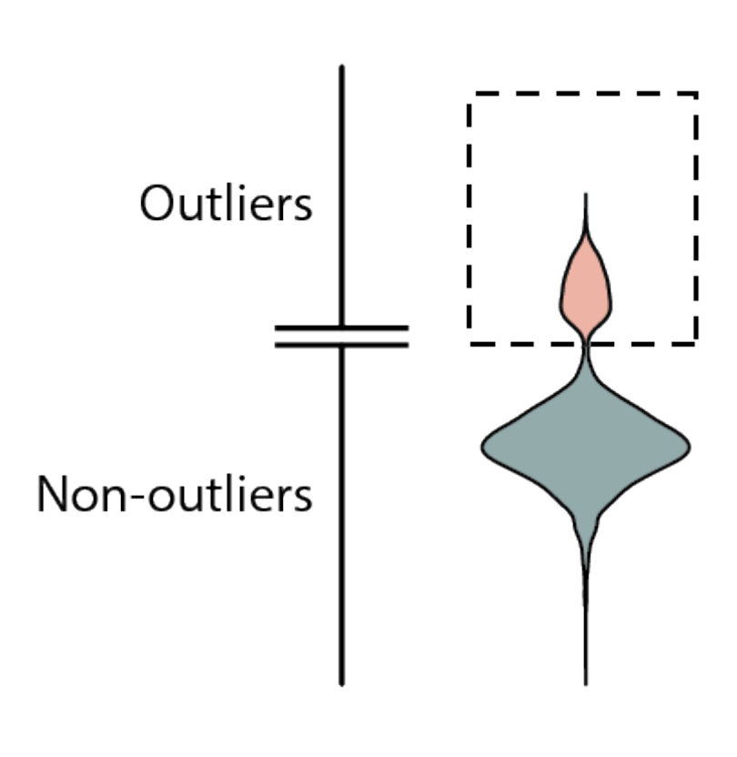
A violin plot combines a box plot and a density plot. It displays the distribution of the data as well as its density.
The central box represents the interquartile range (IQR) like in a box plot.
The “violins” on either side show the density of data at different values.
Points outside the dense areas of the plot can be potential outliers.

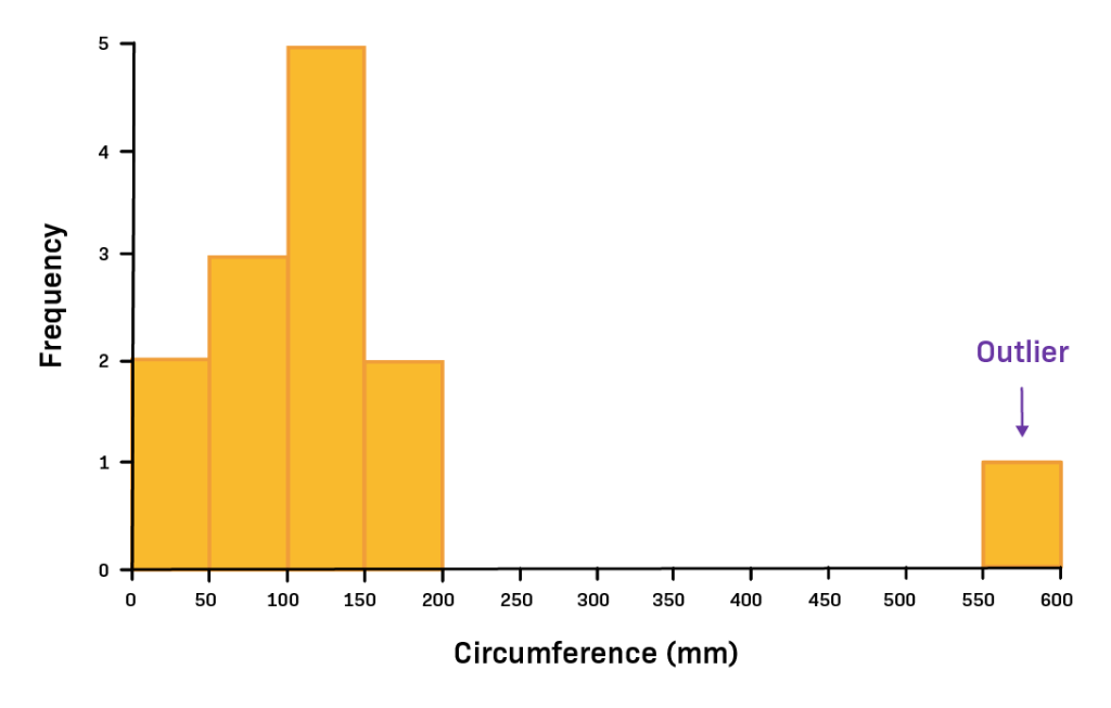
Histogram:

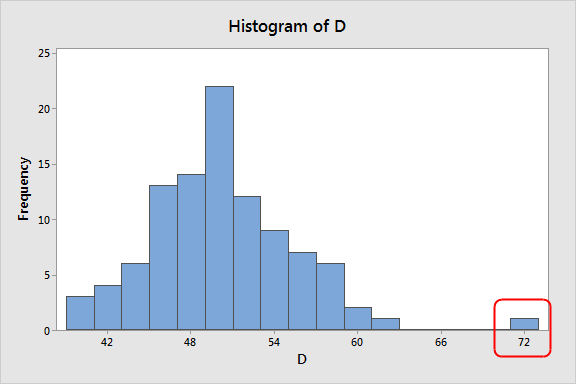
Histograms display the distribution of a single variable by grouping data into intervals or “bins” along the x-axis and showing the frequency of data points in each bin along the y-axis.
Outliers in a histogram can be detected if they fall into bins that have very few data points compared to the other bins.
If a histogram shows a long tail extending beyond the main distribution, those data points in the tail might be outliers.

Finding outliers by some mathematical methodology:

Standard Deviation
Z-Score
IQR

Standard Deviation:

The standard deviation is a measure of how spread out the data is from the mean. Detecting outliers using the standard deviation method involves identifying data points that are located far away from the mean, beyond a certain number of standard deviations.

Steps to Detect Outliers:

Calculate the Mean and Standard Deviation:

First, calculate the mean (average) and standard deviation of the dataset.

Determine the Threshold:

Decide how many standard deviations away from the mean you consider as a threshold for identifying outliers. The standard practice is to use 2 or 3 standard deviations.

Calculate the Cutoff Points:

Multiply the standard deviation by the chosen threshold and then add or subtract this value from the mean to calculate the cutoff points.

Identify Outliers:

Any data point that is beyond the calculated cutoff points is considered an outlier.

Example:

Let’s say you have a dataset of exam scores for a class of students:

Scores: 85, 89, 90, 88, 92, 87, 94, 100, 85, 91

Step 1: Calculate the Mean and Standard Deviation

Mean (μ) = (85 + 89 + 90 + 88 + 92 + 87 + 94 + 100 + 85 + 91) / 10 = 89.1

Next, calculate the differences between each score and the mean, square those differences, and calculate the average of the squared differences. This average is the variance. The standard deviation (σ) is the square root of the variance.

Standard Deviation (σ) = √[ (Σ(xi – μ)^2) / N ]

Step 2: Determine the Threshold

Let’s use a threshold of 2 standard deviations from the mean.

Step 3: Calculate the Cutoff Points

Upper Cutoff Point = Mean + (2 * Standard Deviation)
Lower Cutoff Point = Mean – (2 * Standard Deviation)
Upper Cutoff Point = 89.1 + (2 * σ)
Lower Cutoff Point = 89.1 – (2 * σ)

Step 4: Identify Outliers

Any score greater than the Upper Cutoff Point (≈ 93.4) is considered an outlier.
Any score less than the Lower Cutoff Point (≈ 84.8) is considered an outlier.

IQR:

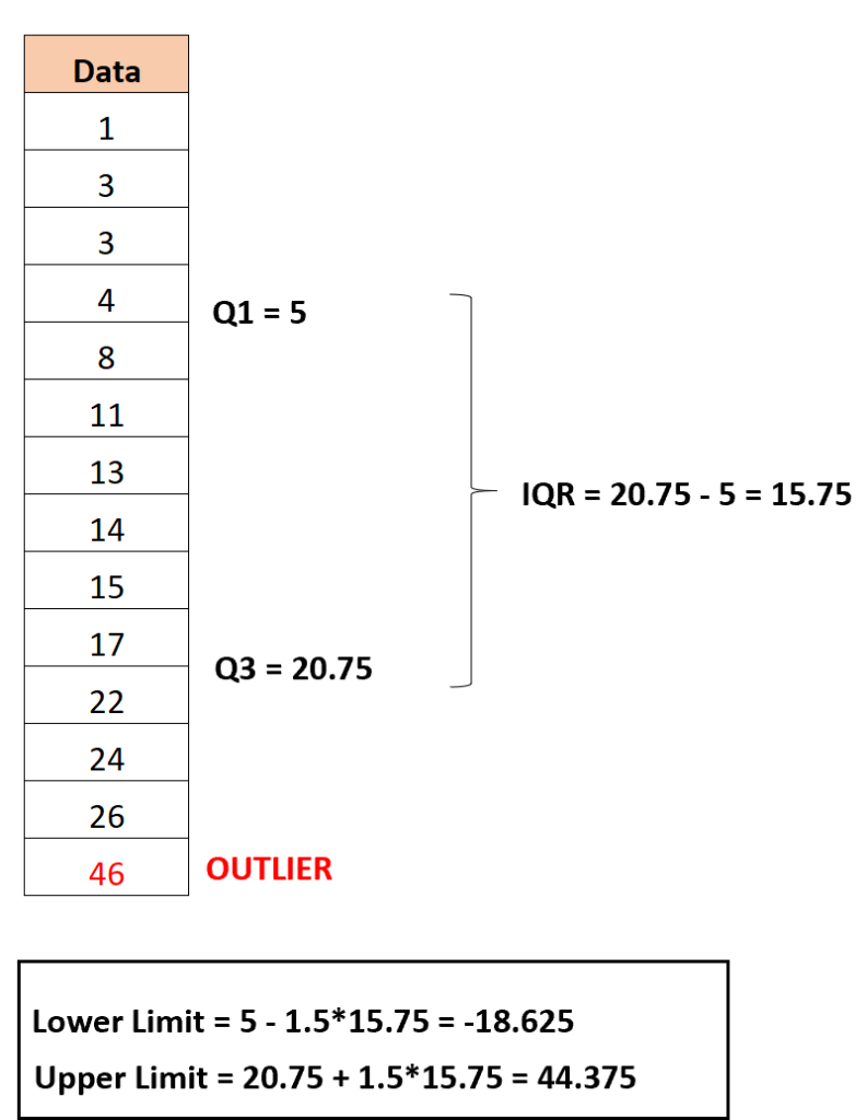
The Interquartile Range (IQR) is a measure of the spread of data in a dataset. It’s based on quartiles, which divide the data into four parts. Detecting outliers using the IQR method involves identifying data points that are located far away from the main body of the data, beyond a certain range determined by the IQR.

Steps to Detect Outliers Using IQR:

Sort the Data:

Start by sorting the dataset in ascending order.

Calculate the Quartiles:

Calculate the first quartile (Q1) and the third quartile (Q3) of the dataset. Q1 represents the value below which 25% of the data falls, and Q3 represents the value below which 75% of the data falls.

Calculate the IQR:

Calculate the IQR by subtracting Q1 from Q3:

IQR = Q3 – Q1.

Determine the Cutoff Points:

Multiply the IQR by a factor (often 1.5) and use this value to determine the cutoff points for potential outliers.

Identify Outliers:

Any data point that is less than Q1 – (1.5 * IQR) or greater than Q3 + (1.5 * IQR) is considered an outlier.

Example:

Let’s use the same dataset of exam scores for a class of students:

Scores: 85, 89, 90, 88, 92, 87, 94, 100, 85, 91

Step 1: Sort the Data

Sorted Scores: 85, 85, 87, 88, 89, 90, 91, 92, 94, 100

Step 2: Calculate the Quartiles

Q1 = 87 (the median of the lower half: 85, 85, 87, 88, 89)
Q3 = 92 (the median of the upper half: 90, 91, 92, 94, 100)

Step 3: Calculate the IQR

IQR = Q3 – Q1 = 92 – 87 = 5

Step 4: Determine the Cutoff Points

Upper Cutoff Point = Q3 + (1.5 * IQR) = 92 + (1.5 * 5) = 99.5
Lower Cutoff Point = Q1 – (1.5 * IQR) = 87 – (1.5 * 5) = 79.5

Step 5: Identify Outliers

Any score greater than the Upper Cutoff Point (≈ 99.5) is considered an outlier.
Any score less than the Lower Cutoff Point (≈ 79.5) is considered an outlier.

Z-Score:

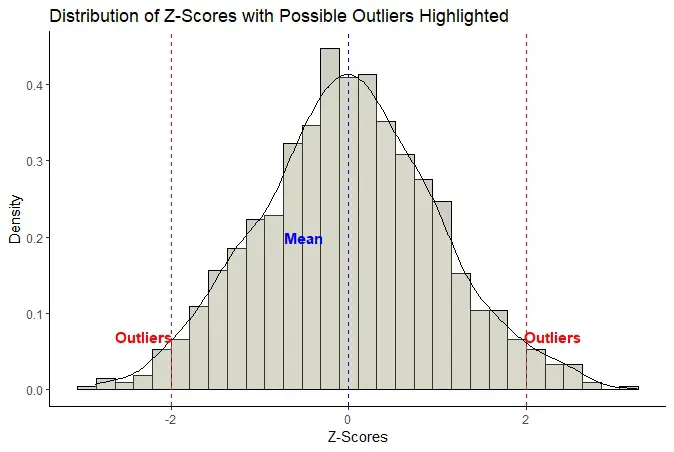
The Z-score is a statistical measure that quantifies how far a data point is from the mean in terms of standard deviations. Detecting outliers using the Z-score method involves calculating the Z-score for each data point and identifying those that are significantly distant from the mean.

Steps to Detect Outliers Using Z-Score:

Calculate the Mean and Standard Deviation:

Start by calculating the mean (average) and standard deviation of the dataset.

Calculate the Z-Score for Each Data Point:

Calculate the Z-score for each data point using the formula:

Z = (X – μ) / σ

Where:

Z is the Z-score
X is the data point
μ is the mean
σ is the standard deviation

Determine the Threshold:

Decide on a threshold Z-score value beyond which you consider data points to be outliers. A common choice is a Z-score of 2 or 3.

Identify Outliers:

Any data point with a Z-score greater than the chosen threshold is considered an outlier.

Example:

Let’s use the same dataset of exam scores for a class of students:

Scores: 85, 89, 90, 88, 92, 87, 94, 100, 85, 91

Step 1: Calculate the Mean and Standard Deviation

Mean (μ) = (85 + 89 + 90 + 88 + 92 + 87 + 94 + 100 + 85 + 91) / 10 = 89.1
Next, calculate the standard deviation (σ) as explained before.

Step 2: Calculate the Z-Score for Each Data Point

Z = (X – μ) / σ

For each data point:

Z-score for 85: (85 – 89.1) / σ
Z-score for 89: (89 – 89.1) / σ
… and so on for each score

Step 3: Determine the Threshold

Let’s use a threshold Z-score of 2.

Step 4: Identify Outliers

Any score with a Z-score greater than 2 (or another threshold you choose) is considered an outlier.

Dealing with these outliers:

By imputation, we can overcome from this issue, and to impute, we have several techniques like imputation by mean, mode, median, 0, 1, and K-Imputers. Let’s see one by one.

Mean:

When dealing with outliers, one approach is to replace the outlier values with the mean value of the rest of the data. This method can help mitigate the impact of outliers on statistical analysis or modeling.

Let’s say you have a dataset with outliers:

Data: [12, 15, 18, 25, 20, 30, 110, 22, 19]

Step 1: Identify Outliers

Suppose you use the Z-score method and identify 110 as an outlier.

Step 2: Calculate the Mean

Calculate the mean of the dataset without the outlier (110):

Mean = (12 + 15 + 18 + 25 + 20 + 30 + 22 + 19) / 8 = 21.125

Step 3: Replace Outliers

Replace the outlier (110) with the calculated mean value (21.125):
Data (with replaced outlier): [12, 15, 18, 25, 20, 30, 21.125, 22, 19]

Benefits and Considerations:

Impact Reduction: Replacing outliers with the mean can help reduce the influence of extreme values on statistical measures like the mean and standard deviation.
Maintaining Data Structure: Imputing with the mean preserves the overall structure of the dataset.
Potential Biases: However, imputing with the mean can introduce biases, especially if the outliers represent genuine patterns in the data.
Sensitive to Outliers: This method doesn’t eliminate the impact of outliers; instead, it redistributes their influence.