Mastering Optimization: Dynamic Learning Rates Unveiled
Definition of Traditional Optimization Functions:- Traditional optimization functions are mathematical algorithms and techniques used in machine learning to fine-tune model parameters during the training process. These functions are essential for the iterative improvement of a machine learning model’s performance by minimizing a predefined loss function.
To better understand traditional optimization functions, let’s break down the key components
Mathematical Optimization
Machine learning models are essentially mathematical functions that map input data to output predictions. Traditional optimization functions help find the optimal set of model parameters (weights and biases) that minimize the difference between these predictions and the actual target values.
Imagine you have a special recipe for making a sandwich. Your goal is to make the tastiest sandwich ever! But, you have some secret ingredients (let’s call them “parameters”) like how much cheese or lettuce to use.
Traditional optimization is like finding the perfect amounts of these secret ingredients to make your sandwich taste the best. We use math to figure out these amounts. It’s like a delicious math problem!
Loss Function
In machine learning, a loss function (also known as a cost function or objective function) quantifies how well the model’s predictions match the actual target values. The goal is to minimize this loss function. Common loss functions include mean squared error for regression tasks and cross-entropy for classification tasks.
Now, imagine you’re the sandwich judge. You taste a sandwich, and you have a special taste-testing scale to measure how far off it is from being perfect. The higher the score, the worse the sandwich tastes.
In machine learning, we have something similar called a “loss function.” It’s like your taste-testing scale. It tells us how far off our predictions are from being perfect. For example, if you predict a test score of 90, but the real score is 95, your loss is 5 points (90 – 95). Our goal is to make the loss as small as possible, like aiming for a score of 0 on your taste-testing scale. When the loss is small, our predictions are close to being perfect!
Iterative Process
Model training is an iterative process. Traditional optimization functions work by adjusting model parameters slightly in each iteration to reduce the loss. This process continues until the model converges to a state where further adjustments do not significantly improve performance.
Now, let’s talk about making your sandwich even better. You start by adding a bit more cheese and taking away some mustard. You taste it again and see if it’s getting closer to perfection. If it is, you keep making those changes. But, if you’ve gone too far and it tastes worse, you go back a step.
In machine learning, we do something similar. We start with random guesses (like adding random amounts of cheese and mustard to your sandwich). Then, we use our loss function to see how bad our guesses are. We make small adjustments to our guesses to make them better, just like tweaking your sandwich.
We keep doing this over and over until our loss (how far off we are from perfection) is as small as possible. It’s like making tiny improvements to your sandwich until it’s the tastiest sandwich ever!
Let’s say you’re predicting grades for a math test. Your model starts with random guesses for each student’s grade. The loss function checks how wrong your guesses are compared to the real grades.
- Student 1: Real grade = 90, Model’s guess = 80
- Student 2: Real grade = 85, Model’s guess = 75
- The loss function adds up these differences: (90 – 80) + (85 – 75) = 10 + 10 = 20.
- The goal is to minimize this loss. Imagine you can tweak your model’s guesses. You could increase Student 1’s guess to 85 and Student 2’s guess to 80.
- Now, the loss becomes (90 – 85) + (85 – 80) = 5 + 5 = 10.
- By adjusting the guesses (like optimizing your throws), you reduced the loss, and your model is better at predicting grades.
Significance of Traditional Optimization Functions
Convergence
Optimization functions ensure that a machine learning model converges to an optimal state, where it performs well on the given task. Without optimization, models would not learn from data effectively.
Generalization
Effective optimization helps prevent overfitting, where a model performs well on the training data but poorly on new, unseen data. By minimizing the loss function, optimization functions promote model generalization.
Efficiency
Optimization functions guide the training process efficiently by finding the steepest descent direction in the loss landscape. This means they make the most significant improvements to the model with each step.
Scalability
Traditional optimization functions are scalable and can handle a wide range of machine learning problems, from simple linear regression to complex deep neural networks. They provide a universal framework for parameter tuning.
Interpretability
Many traditional optimization algorithms are interpretable, meaning they provide insights into how and why a model is adjusting its parameters. This can be crucial for debugging and understanding model behavior.
Challenges with Traditional Optimization Functions
Traditional optimization functions are powerful tools for training machine learning models, but they are not without their challenges and limitations. One of the most critical challenges is the selection of an appropriate learning rate, which can significantly impact the training process.
Learning Rate and Its Importance
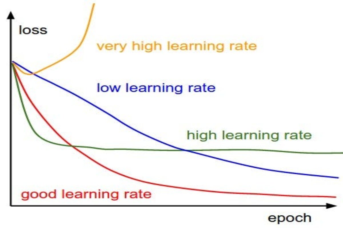
The learning rate is a fundamental hyperparameter in many optimization algorithms, including gradient descent-based methods. It determines the size of the steps taken during each iteration of parameter updates. In simple terms, it decides how fast or slow the model learns from the data.
Now, think of the “learning rate” as how quickly or slowly you’re willing to adjust your balance on the bike as you ride. If you adjust it too fast, you might fall off because you’re making big changes too quickly. If you adjust it too slowly, you might not learn to balance properly because you’re not making enough changes.
The Goldilocks Dilemma
Selecting the right learning rate is often likened to the “Goldilocks dilemma” from the fairy tale. It shouldn’t be too large, or too small, but just right. Here’s why:-
Learning Rate Too Large (Overshooting)
- If the learning rate is set too high, the optimization process can overshoot the optimal parameters. Imagine trying to balance on a tightrope while taking huge steps. You’re likely to miss the balance point and fall off.
- Imagine if you decided to adjust your bike balance quickly while riding. You’d probably wobble and fall off because you’re overcorrecting. This is similar to setting a learning rate too high in machine learning; the model adjusts too much and might not learn properly.
Learning Rate Too Small (Slow Convergence)
- Conversely, if the learning rate is too small, the optimization process progresses very slowly. It’s like taking tiny, almost imperceptible steps on the tightrope. While you won’t fall, it will take a long time to reach the balance point.
- On the other hand, if you barely adjust your balance while riding, you won’t make much progress, and it will take forever to become a good rider. This is like setting a learning rate too low in machine learning; the model learns very slowly.
Impact on Convergence
The learning rate directly affects the convergence of the optimization algorithm. Convergence refers to the process of the model gradually getting closer to the optimal solution, where the loss function is minimized. Achieving convergence quickly and efficiently is a desirable goal in machine learning.
Convergence is like becoming a really good bike rider. It’s when the model gets better and better at its task, and the learning process comes to a stop because it’s reached its best performance.
Fast Convergence
- A well-chosen learning rate can lead to fast convergence, reducing the time it takes for the model to reach a good solution.
- A well-chosen learning rate can help your model learn quickly and become a great performer in a short time. It’s like quickly mastering bike riding and becoming a pro.
Slow Convergence
- An inappropriate learning rate, whether too high or too low, can lead to slow convergence or even convergence to a suboptimal solution.
- If you choose the wrong learning rate, it’s like learning to ride a bike at a snail’s pace. It takes a long time to get good, or you might not even reach your full potential.
Heterogeneous Data and Changing Landscapes
Machine learning models often deal with diverse and complex datasets. Different parts of the dataset may have different characteristics, and the landscape of the loss function can change during training. Traditional optimization functions, which use a fixed learning rate, may struggle to adapt to these variations.
Heterogeneous Data
- When dealing with data with varying scales or importance, a fixed learning rate may cause difficulties. For example, one feature in your data may have values in the range of 1 to 10, while another feature has values in the range of 1000 to 10000. A fixed learning rate might work well for one but poorly for the other.
- Some data features might be small and easy to handle (like riding on a smooth road), while others might be huge and challenging (like riding on a bumpy path). Choosing a single learning rate might not work well for all parts of your data.
Changing Loss Landscape
- The loss landscape, which represents how the loss function behaves concerning model parameters, can be complex and change as the optimization progresses. Traditional optimization functions may find it challenging to navigate this changing landscape optimally.
- Imagine you’re learning how to ride a bike, and you want to get good at it. You know that one of the keys to becoming an excellent bike rider is finding the right balance. However, finding that perfect balance isn’t as easy as it sounds.
- The “loss landscape” in machine learning is like the different challenges you encounter while riding your bike. It’s the ups and downs of the terrain. Traditional optimization functions have a fixed learning rate, which can be like trying to ride your bike at the same speed on all types of roads. Sometimes, you need to adjust your learning rate to navigate these changes optimally.
So, just as you learn to balance and ride your bike with different terrains and speeds, machine learning models need the right learning rate to find their balance and become skilled at their tasks. Choosing the perfect learning rate is a bit like finding the sweet spot in your bike riding journey.
Traditional optimization functions may be preferred in specific scenarios
Resource Constraints
In resource-limited settings, such as edge devices or constrained computational environments, traditional functions like SGD can be the pragmatic choice due to their computational efficiency.
Stability Emphasis
When model stability and avoiding divergence are paramount, traditional optimization functions may be favored for their conservative convergence properties.
Interpretable Models
In contexts where interpretability and model transparency are crucial, linear models optimized using traditional methods provide transparency and ease of interpretation.
Introduction to Dynamic Learning Rates
Dynamic learning rates represent a paradigm shift in optimization functions within the realm of machine learning. Instead of employing a static, fixed learning rate throughout the training process, dynamic learning rate techniques adapt this crucial parameter dynamically as optimization unfolds. This adaptability is a response to the ever-present challenge of optimizing complex models effectively.
Motivation Behind Using Dynamic Learning Rates
Adaptation to Data Dynamics
In the real world, data is seldom static; it exhibits intricate dynamics. Different parts of datasets may manifest varying patterns, scales, and noise levels. Dynamic learning rates enable models to flexibly adjust their learning pace to these dynamic data characteristics. For instance, in the face of noisy or rapidly fluctuating data, a larger learning rate can expedite model adaptation, while smaller rates can fine-tune model parameters in more stable data regions. This adaptability aligns the model’s learning process with the inherent complexities of real-world data.
Faster Convergence
Achieving convergence—the state where a model effectively minimizes its loss function—is a coveted objective in machine learning. Dynamic learning rates, by their ability to adapt, contribute to the acceleration of convergence during optimization. By varying the learning rate in response to the model’s learning progress, these methods minimize the time required for the model to attain a satisfactory solution. This expedited convergence is particularly valuable in tasks where rapid model deployment or experimentation is imperative.
Stability and Robustness
The stability of the training process is of paramount importance. Dynamic learning rates play a pivotal role in ensuring the stability and robustness of optimization algorithms. They monitor and respond to the intricate nuances of the loss landscape—the topography of the loss function concerning model parameters. By doing so, they effectively avoid scenarios where the optimization process either diverges into instability or converges at an unacceptably slow rate. This characteristic engenders reliability and efficiency in the model training pipeline.
Reduced Hyperparameter Tuning
The process of hyperparameter tuning, especially the selection of an appropriate learning rate, can be an arduous task, often requiring significant manual intervention. Dynamic learning rate methods mitigate this challenge by necessitating fewer hyperparameters to be manually fine-tuned. This simplification streamlines the optimization process and reduces the risk of selecting suboptimal hyperparameters, sparing researchers valuable time and effort.
Implicit Regularization
Implicit regularization, a concept inherent to some dynamic learning rate techniques like Adam, emerges as a desirable byproduct. This form of regularization discourages models from fitting noise in the data. By doing so, it promotes better generalization, enhancing a model’s capacity to perform well on unseen data—a pivotal aspect of machine learning model quality.
Advantages of Dynamic Learning Rate Optimization Functions
Dynamic learning rate optimization functions offer several compelling benefits that make them an attractive choice in the fields of machine learning and deep learning. Let’s explore these advantages:
Learning Rate Challenges
Choosing the right learning rate is a critical aspect of training machine learning models. Traditional optimization functions rely on a fixed learning rate, which can be challenging to determine.
Overshooting Prevention
- Dynamic learning rate methods adaptively adjust the learning rate during training. If it starts too high, they automatically reduce it as needed to prevent overshooting the minimum point of the loss function. This prevents the model from diverging, a situation where it fails to converge to a good solution.
Avoiding Slow Convergence
- On the other hand, if the learning rate is too low in traditional optimization, the convergence can be painfully slow. Dynamic methods can increase the learning rate when progress is slow, leading to faster convergence without the risk of overshooting.
Adaptability to Data
Real-world data is often complex, and different parts of the data may have different characteristics. Dynamic learning rate functions can adapt to these variations, which is particularly advantageous when dealing with messy and dynamic datasets.
Variable Learning Rates
- Dynamic methods can assign larger learning rates to portions of the data that require quick adaptation and smaller rates to stable parts that need fine-tuning. This adaptability helps the model learn efficiently from various data patterns.
Faster Convergence
One of the most significant advantages of dynamic learning rate optimization is its ability to accelerate convergence during model training.
Quick Learning Response
- By adjusting the learning rate based on the model’s learning progress, dynamic methods can speed up convergence. When the model is far from the optimal solution, they allow larger steps, and as it gets closer, they automatically reduce the learning rate. This results in quicker training.
Improved Stability
Dynamic learning rate methods contribute to more stable training processes, which is essential for reliable model development.
Loss Landscape Adaptation
- They react to the loss landscape’s characteristics, making training more robust. If the loss landscape is steep, indicating quick progress, they use a larger learning rate. If it’s flat, indicating slower progress, they use a smaller rate. This adaptability avoids divergence and ensures stable convergence.
Robustness to Hyperparameters
Traditional optimization often requires manual tuning of hyperparameters, including the learning rate. Dynamic learning rate methods reduce this complexity.
Reduced Hyperparameter Tuning
- Many dynamic methods have fewer hyperparameters to tune compared to traditional methods. This simplifies the optimization process and makes it less susceptible to manual tuning errors.
Regularization Effect
Some dynamic learning rate methods, such as Adam, offer a regularization effect that aids in preventing overfitting, a common issue in machine learning.
Implicit Regularization
- Adam implicitly includes regularization by using a moving average of past gradients. This prevents the model from fitting noise in the data and enhances its generalization capability.
Let’s see one example of ‘Learning to Ride a Bike’.
Imagine you’re learning how to ride a bike, and you want to become a skilled bike rider. You know that one of the keys to mastering bike riding is finding the right balance on two wheels. However, finding that perfect balance isn’t as easy as it sounds.
Fixed Learning Rate
First, let’s consider what it would be like if you had a fixed learning rate for your bike riding lessons. In this case, you decide that you’ll always pedal at the same speed, no matter what.
Challenge 1
- Learning on Uneven Ground: When you start practicing on an uneven or bumpy road, your fixed learning rate doesn’t adapt. You keep pedaling at the same speed, and as a result, you struggle to maintain balance. You might even fall off the bike because you’re not adjusting to the changing terrain.
Challenge 2
- Progressing Too Slowly: On the other hand, when you ride on a smooth, flat road, your fixed learning rate still stays the same. This means you’re not taking full advantage of the easy terrain to build your skills quickly. You’re progressing too slowly because you’re not adapting to the easier conditions.
Challenge 3
- Risk of Falling: Your fixed learning rate doesn’t respond well to your learning progress. If you’re wobbly and unsteady, it doesn’t slow down to help you regain balance. As a result, you might fall off the bike more often because it doesn’t adapt to your skill level.
Dynamic Learning Rate
Now, let’s introduce the concept of a dynamic learning rate to your bike riding lessons. With a dynamic learning rate, you’re more like a flexible learner.
Adaptation to Terrain
- When you’re on a bumpy road, your dynamic learning rate adjusts. It’s like you instinctively slow down when you hit rough patches to maintain balance. This adaptability helps you navigate tricky terrains without falling off.
Optimal Learning Speed
- On a smooth, flat road, your dynamic learning rate recognizes that you don’t need to pedal too hard to maintain balance. It allows you to ride comfortably and learn at an optimal speed. You’re not wasting energy because your learning rate is in tune with the situation.
Balancing Act
- If you start wobbling or losing balance, your dynamic learning rate senses the struggle and slows down just enough to help you regain your balance. It’s like having a built-in stabilizer that kicks in when you need it most.
Learning Rate Schedules
Learning rate schedules are strategies used in machine learning to adjust the learning rate during training. These schedules help optimize the training process by adapting the learning rate based on predefined rules. Three common learning rate schedules are step decay, exponential decay, and cyclic learning rates.
Step Decay
This schedule involves reducing the learning rate at predefined intervals or steps during training. For example, you might decrease the learning rate by half every 10 epochs. This adapts the learning rate to the training progress and data patterns, slowing it down to fine-tune the model when needed.
Exponential Decay
Exponential decay gradually decreases the learning rate over time. It starts with a higher learning rate and reduces it exponentially during training. This schedule ensures faster learning initially and fine-tuning as training progresses. It’s like gradually learning to control your bike’s speed as you gain experience.
Cyclic Learning Rates
Cyclic learning rates dynamically change the learning rate during training cycles. They allow the learning rate to vary in response to the model’s performance and data characteristics. For instance, the learning rate might increase during steep learning curves and decrease when progress slows down. This adaptation helps the model efficiently navigate complex data landscapes.
In essence, learning rate schedules serve as guiding strategies to tailor the learning rate to the needs of the model and the data, promoting more efficient and effective training. They are like having a coach who adjusts your training pace based on your progress and the challenges you encounter, ensuring that you reach your training goals effectively.
Implementing Dynamic Learning Rates in TensorFlow and PyTorch
Dynamic learning rates play a pivotal role in optimizing the training of machine learning models. They adapt to the evolving characteristics of data and the learning progress of the model. Implementing dynamic learning rates in popular frameworks like TensorFlow and PyTorch involves a systematic process:
Choose a Dynamic Learning Rate Schedule
Before embarking on implementation, decide upon the learning rate schedule that best suits your problem. Common schedules include step decay, exponential decay, and cyclic learning rates. Each schedule has unique properties tailored to different scenarios.
Import Necessary Libraries
In both TensorFlow and PyTorch, it’s imperative to import the requisite libraries and modules. In TensorFlow, you can leverage ‘tensorflow’ or ‘tf.keras,’ while in PyTorch, you’ll primarily interact with ‘torch’ and ‘torch.optim.’
Define the Learning Rate Schedule
Create a function or class that defines your chosen learning rate schedule. This function typically takes parameters such as the current epoch or iteration number and returns the learning rate corresponding to that point in training. The schedule’s design should align with the dynamics of your data and problem.
Configure the Optimizer
In TensorFlow
- Choose your optimizer, for example, ‘tf.keras.optimizers.Adam.’
- Set the initial learning rate to the output of your learning rate schedule function.
- You may use ‘tf.keras.optimizers.schedules.LearningRateSchedule’ if your schedule is epoch or step-based.
In PyTorch
- Select the optimizer, like ‘torch.optim.SGD’ or ‘torch.optim.Adam.’
- Initialize the optimizer with the initial learning rate.
- You can manually adjust the learning rate during training by modifying the optimizer’s ‘param_groups.’
Training Loop
- Construct a training loop where you iterate through epochs or batches of data.
- At each epoch or step, invoke your learning rate schedule function to acquire the current learning rate.
- Update the optimizer’s learning rate with the newly obtained value.
Monitoring and Visualization
During the training process, it’s pivotal to monitor the behavior of the dynamic learning rate. You can log or visualize the rate’s progression over time to ensure it adapts as anticipated.
Experimentation
Hyperparameter tuning is an essential step. Experiment with various learning rate schedules and associated parameters to ascertain the best model performance. This often necessitates empirical experimentation to determine the most suitable settings.
Resources
Refer to the official documentation of TensorFlow and PyTorch for comprehensive tutorials and detailed examples of implementing dynamic learning rates in various scenarios. Both frameworks provide abundant resources to guide you through the process.
Conclusion
In your bike riding journey, the concept of dynamic learning rates is akin to having a bike that adjusts its speed and stability based on the road conditions and your skill level. It adapts to keep you balanced, helps you learn at the right pace, and reduces the risk of falling. Similarly, in machine learning, dynamic learning rates adapt to data complexities and model learning progress, making the training process more efficient and reliable.


