The Decision tree algorithm is a type of supervised machine learning. This is a tree-based algorithm. As per the name, the model draws a tree. To build a tree, model partitions the data, and then use an if-else question-answering strategy, and with each answer, the model decides the tree will grow or stop. Trees grow with branches and stop with the leaf nodes which is the last stage of the tree. This tree grows until finds the final leaf node, therefore, decision tree has always been good for training. But it is not as much generalized for testing, since most of the time, we face the overfitting issue with decision tree algorithm.
It is a parametric algorithm. The distribution of a tree is similar to real-life trees. It start with the root node, grow with branches, and stop with the leaf node. A leaf node represents a prediction. Decision trees are used for both classification and regression, but they most commonly used for classification.
Why? Let’s see:
Intuitive representation:
- It offers a straightforward and intuitive way to classify the data points.
- The branch represents independent variables, and because of this structure, the decision tree is very easy to understand.
- Non-technical people can easily understand how classification is going to take place.
Efficiently handle both binary and multi-classification:
- Naturally, it tends to binary classification.
- But decision trees can easily handle multiclass classification by creating multiple branches.
Handles any type of data:
- Decision tree don’t require any specific format of data to run, they can run on both linear and non-linear data efficiently.
————————————————————————————————————————————————————————————————-
That’s why a decision tree is mostly preferable for classification, but there is no such thumb rule for this, we can also use a decision tree for regression efficiently. Decision trees provide valuable information about features, for example which node is near the root, that node is very important, and which is far away from the root, that node is having low importance. As I mentioned earlier said, due to efficient generalization with training data, and not that much with testing data, the decision tree tends to overfit, let’s look at how overfitting happens with one simple example.
Suppose, we have a dataset 1000 entries, which includes information about apples and oranges, having only two features: 1. Color and 2. Weight.
Now in the above feature, we got know that all apples are red and their weight is not more than 145 grams. And all oranges are not red and each orange’s weight is more than 145 grams. Based on this detail, the model draws a tree., because as training data, the model learns all things very well.
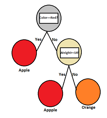
Now time for testing, suppose we have one orange whose weight is less than 145 grams.
In the first node, is colour == red?
The answer will be no.
(Then come next branch)
In the second node, Is weight <=145 grams?
Answer Yes.
But due to tree growth, the model predicts that the orange is an apple (Because all apples below weigh 145 grams). This is nothing but the overfitting, The model learns very well on training data, but it doesn’t perform that well on testing data.
To avoid this, in the decision tree, we use some techniques, like:
Use of Hyperparameter tuning:
- Max_Depth >> None
- Min_Sample_split >> 2 (Branch Node)
- Min_Sample_leaf >> 1 (leaf node)
- Criteria >> ‘Gini’ or (‘Entropy’)
If we set,
- Max_Depth >> High >> Overfitting
- Max_Depth >> Low >> Underfitting
Use of Pruning:
- Pre-Pruning
- Post-Pruning
Using some next version’s algorithms:
- Ada Boost
- Random Forest
—————————————————————————————————————————————————————————————————-
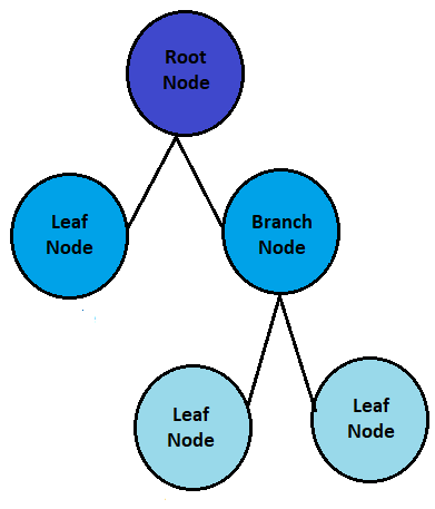
The decision tree has a three types of nodes: the root node, branch node, and the leaf node let’s see all.
Root Node:
- It is the topmost feature of the decision tree
- It represents the entire dataset that we want to use for classification.
- The root node does not have any incoming arrows because it is the starting point of the trees.
Branch node:
- This is an impure node
- It is also known as an internal node, which has an incoming arrow from the parent node and an outgoing arrow for the child node.
For example:
When classifying the fruits based on color and weight, the model asks the question like, is the color red..? This question turns into the branch. That means color and weight are the branches of the model.
Leaf Node:
- This is the pure node because this is the last node of the tree, and after the leaf node, no growth takes place.
- It can also be known as a terminal node, which means it does not have any child node, The leaf node provides optimal decision or prediction.
These three nodes are hierarchical features of the decision tree, which are enable making decision based on different features and splitting data into meaningful subsets for accurate predictions.
—————————————————————————————————————————————————————————————————-
To split the dataset, decision tree has 2 criteria:
- Entropy
- Gini Value
Entropy:
- It is used to find the impurity between nodes. It is a metric, used to measure the impurity of the node.
- We denote Entropy as H(s) or E(s). It ranges between 0 to log2.
- 0 = Pure
- Maximum = Impure.
- We need to find the entropy of each attribute, once it is completed, we go on to find the best root node. To find the best root node, we require Information gain.
Information gain:
- It is a measurement through which we can measure the changes in entropy.
- It decides which attributes should be selected as the root node or decision node.
- Information gain selects the attribute with the highest value of entropy as the root node.
- At the background of the information ground, ID3 (Iterative Dichotomiser algorithm works).
—————————————————————————————————————————————————————————————————-
Let’s look at how Entropy works mathematically.
Let’s assume we have a dataset of 12 fruits with the following features: “color,” “size,” and “sweetness,” and their corresponding labels as “Apple” or “Orange.” The dataset is as follows:
| Apple | Red | Small | Medium |
| Orange | Red | Small | Medium |
| Apple | Red | Small | High |
| Orange | Yellow | Medium | High |
| Orange | Green | Medium | High |
| Apple | Yellow | Small | Medium |
| Orange | Red | Medium | Low |
| Apple | Yellow | Large | High |
| Orange | Red | Medium | Medium |
| Apple | Green | Large | High |
| Orange | Yellow | Large | Medium |
| Orange | Red | Small | High |
Now, let’s build the decision tree step by step using Entropy and Gini index:
Step 1: Calculate the Entropy of the Whole Dataset:
Number of Apples (A) = 5
Number of Oranges (O) = 7
Entropy (H(parent)) = – [(A/total) * log2(A/total) + (O/total) * log2(O/total)]
= – [(5/12) * log2(5/12) + (7/12) * log2(7/12)]
≈ 0.9988
—————————————————————————————————————————————————————————————————-
Step 2: Calculate Information Gain for “Colour” Feature:
Number of Red fruits = 5 (Apples: 3, Oranges: 2)
Number of Green fruits = 3 (Apples: 1, Oranges: 2)
Number of Yellow fruits = 4 (Apples: 1, Oranges: 3)
Information Gain (IG) = H(parent) – [ (Red/total) * H(Red) + (Green/total) * H(Green) + (Yellow/total) * H(Yellow) ]
≈ 0.9988 – [ (5/12) * H(Red) + (3/12) * H(Green) + (4/12) * H(Yellow) ]
Step 2.1: Calculate Entropy for “Red” Fruits:
Number of Apples = 3
Number of Oranges = 2
Entropy (H(Red)) = – [(3/5) * log2(3/5) + (2/5) * log2(2/5)]
≈ 0.97095
Step 2.2: Calculate Entropy for “Green” Fruits:
Number of Apples = 1
Number of Oranges = 2
Entropy (H(Green)) = – [(1/3) * log2(1/3) + (2/3) * log2(2/3)]
≈ 0.9183
Step 2.3: Calculate Entropy for “Yellow” Fruits:
Number of Apples = 1
Number of Oranges = 3
Entropy (H(Yellow)) = – [(1/4) * log2(1/4) + (3/4) * log2(3/4)]
≈ 0.81128
Now, we can calculate the Information Gain for the “Colour” feature:
IG(Color) = 0.9988 – [ (5/12) * 0.97095 + (3/12) * 0.9183 + (4/12) * 0.81128 ]
≈ 0.14304
—————————————————————————————————————————————————————————————————-
Step 3: Calculate Information Gain for “Size” Feature:
Let’s continue building the decision tree by calculating the Information Gain for the “Size” feature:
Number of Small fruits = 3 (Apples: 2, Oranges: 1)
Number of Medium fruits = 6 (Apples: 2, Oranges: 4)
Number of Large fruits = 3 (Apples: 1, Oranges: 2)
Information Gain (IG) = H(parent) – [ (Small/total) * H(Small) + (Medium/total) * H(Medium) + (Large/total) * H(Large) ]
≈ 0.9988 – [ (3/12) * H(Small) + (6/12) * H(Medium) + (3/12) * H(Large) ]
Step 3.1: Calculate Entropy for “Small” Fruits:
Number of Apples = 2
Number of Oranges = 1
Entropy (H(Small)) = – [(2/3) * log2(2/3) + (1/3) * log2(1/3)]
≈ 0.9183
Step 3.2: Calculate Entropy for “Medium” Fruits:
Number of Apples = 2
Number of Oranges = 4
Entropy (H(Medium)) = – [(2/6) * log2(2/6) + (4/6) * log2(4/6)]
≈ 0.9183
Step 3.3: Calculate Entropy for “Large” Fruits:
Number of Apples = 1
Number of Oranges = 2
Entropy (H(Large)) = – [(1/3) * log2(1/3) + (2/3) * log2(2/3)]
≈ 0.9183
Now, we can calculate the Information Gain for the “Size” feature:
IG(Size) = 0.9988 – [ (3/12) * 0.9183 + (6/12) * 0.9183 + (3/12) * 0.9183 ]
≈ 0.0
—————————————————————————————————————————————————————————————————-
Step 4: Calculate Information Gain for “Sweetness” Feature:
Number of Low sweetness fruits = 2 (Apples: 1, Oranges: 1)
Number of Medium sweetness fruits = 5 (Apples: 1, Oranges: 4)
Number of High sweetness fruits = 5 (Apples: 3, Oranges: 2)
Information Gain (IG) = H(parent) – [ (Low/total) * H(Low) + (Medium/total) * H(Medium) + (High/total) * H(High) ]
≈ 0.9988 – [ (2/12) * H(Low) + (5/12) * H(Medium) + (5/12) * H(High) ]
Step 4.1: Calculate Entropy for “Low” Sweetness Fruits:
Number of Apples = 1
Number of Oranges = 1
Entropy (H(Low)) = – [(1/2) * log2(1/2) + (1/2) * log2(1/2)]
= 1.0
Step 4.2: Calculate Entropy for “Medium” Sweetness Fruits:
Number of Apples = 1
Number of Oranges = 4
Entropy (H(Medium)) = – [(1/5) * log2(1/5) + (4/5) * log2(4/5)]
≈ 0.72193
Step 4.3: Calculate Entropy for “High” Sweetness Fruits:
Number of Apples = 3
Number of Oranges = 2
Entropy (H(High)) = – [(3/5) * log2(3/5) + (2/5) * log2(2/5)]
≈ 0.97095
Now, we can calculate the Information Gain for the “Sweetness” feature:
IG(Sweetness) = 0.9988 – [ (2/12) * 1.0 + (5/12) * 0.72193 + (5/12) * 0.97095 ]
≈ 0.12647
Based on the calculated Information Gains, we can see that the “Size” feature has the lowest Information Gain (0.0), which means it doesn’t help us much in separating the fruits into different classes. So, we will choose the “Color” feature as the first split in the decision tree.
—————————————————————————————————————————————————————————————————-
Gini value:
It is also used to find the impurity.
- The Gini value’s range comes between range 0 to 1
- 0= pure
- The lowest value of Gini is considered for selecting the best root node.
- At the background of the Gini value, the CART (Classification and Regression Tree) algorithm is used to select the best root node.
Let’s look at how the Gini value works mathematically.
—————————————————————————————————————————————————————————————————-
Step 1: Calculate the Gini Index of the Whole Dataset:
Number of Apples (A) = 5
Number of Oranges (O) = 7
Gini Index (G(parent)) = 1 – [(A/total)^2 + (O/total)^2]
= 1 – [(5/12)^2 + (7/12)^2]
≈ 0.4959
—————————————————————————————————————————————————————————————————-
Step 2: Calculate Gini Index for “Color” Feature:
Number of Red fruits = 5 (Apples: 3, Oranges: 2)
Number of Green fruits = 3 (Apples: 1, Oranges: 2)
Number of Yellow fruits = 4 (Apples: 1, Oranges: 3)
Gini Index (G) = 1 – [ (Red/total)^2 + (Green/total)^2 + (Yellow/total)^2 ]
≈ 1 – [ (5/12)^2 + (3/12)^2 + (4/12)^2 ]
Step 2.1: Calculate Gini Index for “Red” Fruits:
Number of Apples = 3
Number of Oranges = 2
Gini Index (G(Red)) = 1 – [ (Apples/total)^2 + (Oranges/total)^2 ]
≈ 1 – [ (3/5)^2 + (2/5)^2 ]
≈ 0.48
Step 2.2: Calculate Gini Index for “Green” Fruits:
Number of Apples = 1
Number of Oranges = 2
Gini Index (G(Green)) = 1 – [ (Apples/total)^2 + (Oranges/total)^2 ]
≈ 1 – [ (1/3)^2 + (2/3)^2 ]
≈ 0.4444
Step 2.3: Calculate Gini Index for “Yellow” Fruits:
Number of Apples = 1
Number of Oranges = 3
Gini Index (G(Yellow)) = 1 – [ (Apples/total)^2 + (Oranges/total)^2 ]
≈ 1 – [ (1/4)^2 + (3/4)^2 ]
≈ 0.375
Now, we can calculate the Gini Index for the “Color” feature:
G(Color) = (Red/total) * G(Red) + (Green/total) * G(Green) + (Yellow/total) * G(Yellow)
≈ (5/12) * 0.48 + (3/12) * 0.4444 + (4/12) * 0.375
≈ 0.4278
—————————————————————————————————————————————————————————————————-
Step 3: Calculate Gini Index for “Size” Feature:
Number of Small fruits = 3 (Apples: 2, Oranges: 1)
Number of Medium fruits = 6 (Apples: 2, Oranges: 4)
Number of Large fruits = 3 (Apples: 1, Oranges: 2)
G(Size) = (Small/total) * G(Small) + (Medium/total) * G(Medium) + (Large/total) * G(Large)
≈ (3/12) * 0.4444 + (6/12) * 0.5 + (3/12) * 0.4444
≈ 0.4714
—————————————————————————————————————————————————————————————————-
Step 4: Calculate Gini Index for “Sweetness” Feature:
Number of Low sweetness fruits = 2 (Apples: 1, Oranges: 1)
Number of Medium sweetness fruits = 5 (Apples: 1, Oranges: 4)
Number of High sweetness fruits = 5 (Apples: 3, Oranges: 2)
G(Sweetness) = (Low/total) * G(Low) + (Medium/total) * G(Medium) + (High/total) * G(High)
≈ (2/12) * 0.5 + (5/12) * 0.48 + (5/12) * 0.48
≈ 0.4867
Based on the calculated Information Gain and Gini Index values, we can see that the “Color” feature has the lowest Gini Index (0.4278), and highest Information Gain (0.14304) therefore it gives us the best split for our decision tree.
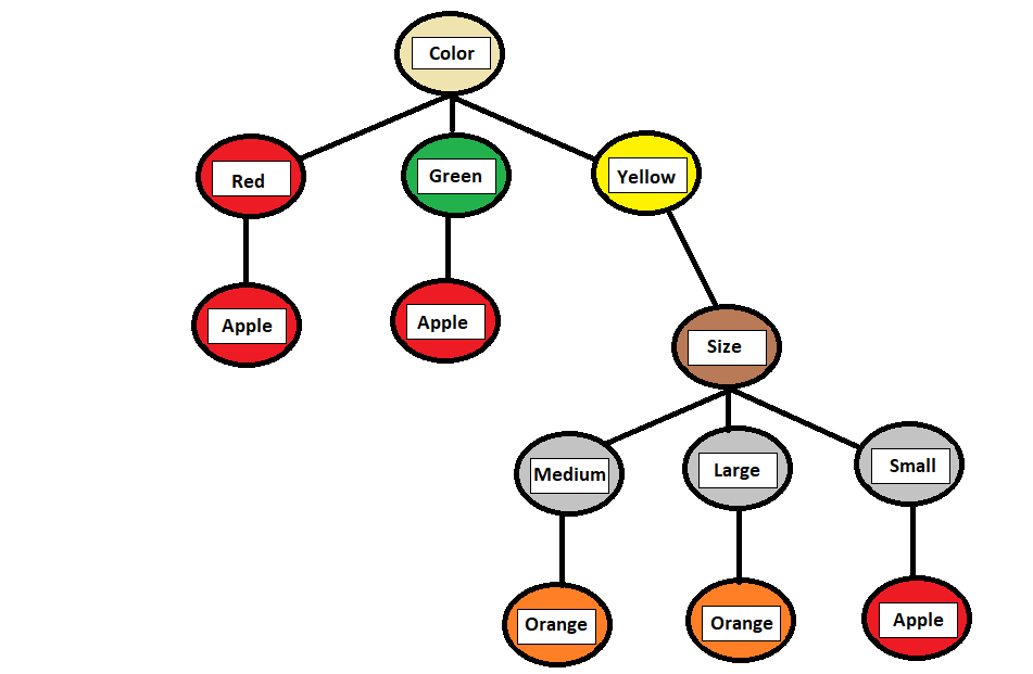
Explanation:
- If the “Colour” is “Red,” it is likely an “Apple.”
- If the “Colour” is “Green,” it is likely an “Apple.”
- If the “Colour” is “Yellow,” it further considers the “Size”:
- If “Medium,” it is likely an “Orange.”
- If “Large,” it is likely an “Orange.”
- If “Small,” it is likely an “Apple.”