StatusNeo

Decision Tree Algorithm- Machine Learning

Overview

Decision Tree Analysis is a general predictive modeling tool. It’s applicable in several different areas. In general, the algorithms identify ways to split a data set based on different conditions. It’s one of the most widely used and practical methods for supervised learning. Decision trees are a supervised learning method that works well for both regression and classification. It uses simple rules to predict the value of a target variable by learning from data features.

Contents

1. What is a Decision Tree?

2. Example of a Decision Tree

3. Entropy/ How Decision Trees Make Decisions?

4. Information Gain

5. When to stop Splitting?

6. How to stop overfitting?

• max_depth
• min_samples_split
• min_samples_leaf
• max_features

7. Pruning

8. Advantage & Disadvantage

WHAT IS A DECISION TREE?

Decision trees can be used for classification and regression problems. The name itself suggests that it uses a flowchart like a tree structure to show the predictions that result from a series of feature-based splits. It starts with a root node and ends with a decision made by leaves.

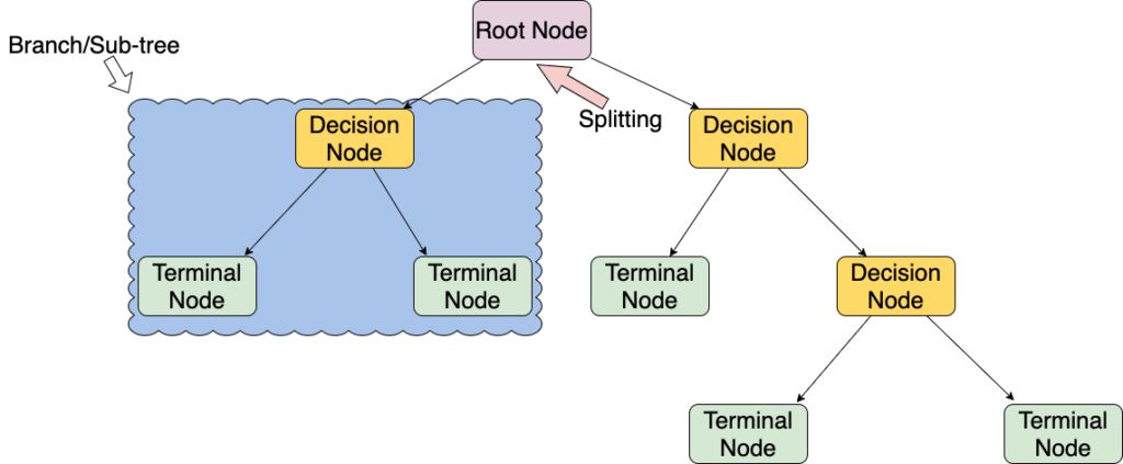
Let’s get familiar with some of the terminologies first.

Root Nodes – It is the node present at the beginning of the decision tree that starts dividing the population into various categories.

Decision Nodes – Decision Nodes are nodes that result after splitting the root nodes.

Leaf Nodes – leaf nodes or terminal nodes are called the nodes where further splitting is impossible.

Sub-tree – a small portion of a graph is called a sub-graph, similarly, a sub-section of this decision tree is called a sub-tree.

Pruning – is nothing but cutting down some nodes to prevent overfitting (something that happens when the machine learns the specific input-output mapping of the training data and extrapolates it to new data).

Example of a decision tree

Decision trees are upside down, so the root is at the top. This root is then split into various nodes. Decision trees are just a bunch of if-else statements in layman’s terms. It checks if the condition is true and if it is, then it goes to the next node attached to that decision.

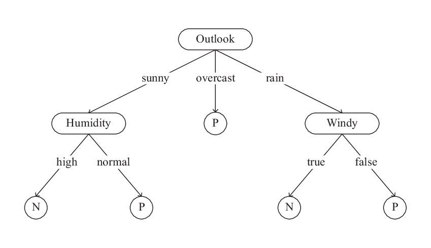
It will go to the next feature which is humidity and wind. It will again check for strong winds or weak winds. If it’s a weak wind and it’s rainy, the person may go and play.

Did you see anything in the above flowchart? We see if the weather is cloudy, we must go to play. Why didn’t it split more? Why did it stop there?

To answer this question, we need to understand a few more concepts like entropy and information gain. But in simple terms, for this training data, I can say that the output is always “yes” for cloudy weather, since there is no disorderliness here we don’t need to split the node further.

The goal of machine learning is to decrease disorder in the dataset. We use decision trees to do this. To decide what should be the root node, there is a metric called “Entropy.” It is the amount of uncertainty in the dataset.

Entropy

Entropy is nothing but the uncertainty in our dataset or measure of disorder. Let me try to explain this with the help of an example.

Suppose you have a group of friends who decides which movie they can watch together on Saturday. There are 2 choices for movies, one is “Conjuring” and the second is “Witch” and now everyone has to tell their choice. After everyone gives their answer we see that “Conjuring” gets 5 votes and “Witch” gets 6 votes. Which movie do we watch now? Isn’t it hard to choose 1 movie now because the votes for both the movies are somewhat equal?

This is exactly what we call disorders, there is an equal number of votes for both the movies, and we can’t really decide which movie we should watch. It would have been much easier if the votes for “Conjuring” were 8 and for “Witch” it was 3. Here we could easily say that the majority of votes are for “Conjuring” hence everyone will be watching this movie.

In a decision tree, the output is mostly “yes” or “no”

The formula for Entropy is shown below:

Here p₊ is the probability of positive class

p_– is the probability of negative class

S is the subset of the training example

How Decision Trees Make Decisions

Now we know what entropy is and what is its formula, Next, we need to know that how exactly does it work in this algorithm.

Entropy basically measures the impurity of a node. Impurity is the degree of randomness; it tells how random our data is. A pure sub-split means that either you should be getting “yes” or “no”.

Suppose a feature has 8 “yes” and 4 “no” initially. After the first split, the left node gets 5 “yes” and 2 “no,” whereas the right node gets 3 “yes” and 2 “no.”

We see here that the split is not pure because we can still have some negative classes in both nodes. In order to make a decision tree, we need to calculate the impurity of each split, and when it’s 100% purity, we make it as a leaf node.

To check the impurity of features 2 and 3 we will take the help of a formula called Entropy.

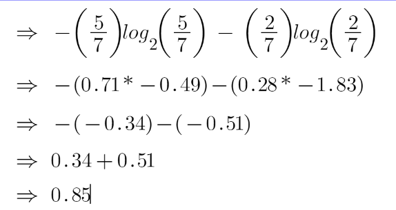
For feature 3,

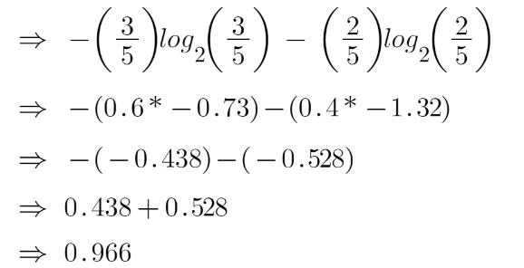
We can see from the tree itself that the left node has low entropy or more purity than the right node since the left node has a greater number of “yes” and it is easy to decide here.

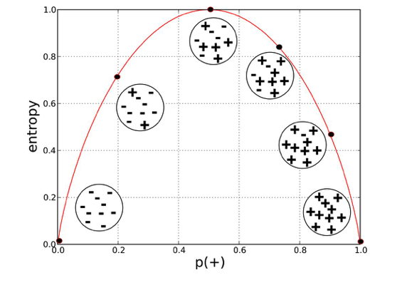
The x and y-axis measure the proportion of data points belonging to the positive class in each bubble and their respective entropies. Right away, you can see an inverted ‘U’ shape of the graph. Entropy is lowest at extremes when the bubble either contains no positive instances or only positive instances. That is, when the bubble is pure its disorder is 0. High entropy occurs in the middle of a bubble chart when the bubble is evenly split between positive and negative instances. The extreme disorder occurs because there is no majority.

Does it matter why entropy is measured using log base 2 or why entropy is measured between 0 and 1 and not some other range? It doesn’t matter. It’s just a metric. It’s important to know how to read it and what it tells us, which we just did above. Entropy is a measure of disorder or uncertainty and the goal of machine learning models and Data Scientists, in general, is to reduce uncertainty.

For this, we bring a new metric called “Information gain” which tells us how much the parent entropy has decreased after splitting it with some feature.

Information Gain

Information gain measures the reduction of uncertainty given some feature and it is also a deciding factor for which attribute should be selected as a decision node or root node.

It is just entropy of the full dataset – entropy of the dataset given some feature.

To understand this better let’s consider an example:

Suppose our entire population had 30 instances. The dataset was to predict whether the person will go to the movie or not. Let’s say 16 people go to the movie and 14 people don’t.

Feature 1 is “Energy” which takes two values “high” and “low”

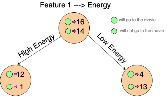
Let’s calculate the entropy:

To see the weighted average of entropy of each node we will do as follows:

Now we have the value of E(Parent) and E(Parent|Energy), information gain will be:

Our parent entropy was near 0.99 and after looking at this value of information gain, we can say that the entropy of the dataset will decrease by 0.37 if we make “Energy” as our root node.

Similarly, we will do this with the other feature 2 “Motivation” and calculate its information gain.

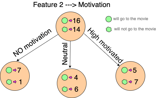
Let’s calculate the entropy here:

To see the weighted average of entropy of each node we will do as follows:

Now we have the value of E(Parent) and E(Parent|Motivation), information gain will be:

We now see that the “Energy” feature gives more reduction than the “Motivation” feature. Thus, we select the feature which has the highest information gain and then split the node based on that feature.

How to stop overfitting?

• max_depth – The higher value of maximum depth causes overfitting, and the lower value causes underfitting.
• min_samples_split – The minimum number of samples required to split an internal node
• min_samples_leaf – The minimum number of samples required to be at a leaf node. A split point at any depth will only be considered if it leaves at least training samples in each of the left and right branches.
• max_features – The number of features to consider when looking for the best split

Pruning

It is another method that can help us avoid overfitting. It helps improve the performance of the tree by cutting the nodes and sub-nodes that aren’t significant. It removes branches that have very low importance.

Advantage & Disadvantage

pros:

1. Its implement flow chart type structure
2. Its help to find all possible outcomes of given problems
3. Handel both numeric and categorical value

cons:

1. Too many layers are extremely complex sometimes.
2. it may result in overfitting.